This chapter introduces two interesting cases of MATLAB image processing: "counting coins" and "Mona Lisa's cat".

(12.1) counting coins

Requirement Description: now there is a picture coins Png, it is required to count the number of coins in the picture with MATLAB.

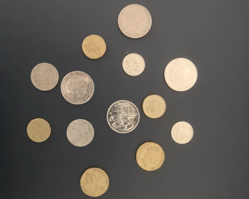
Switch the current folder of MATLAB to install coins PNG file directory, read the picture:

image = imread("coins.png");
imshow(image); %display picture

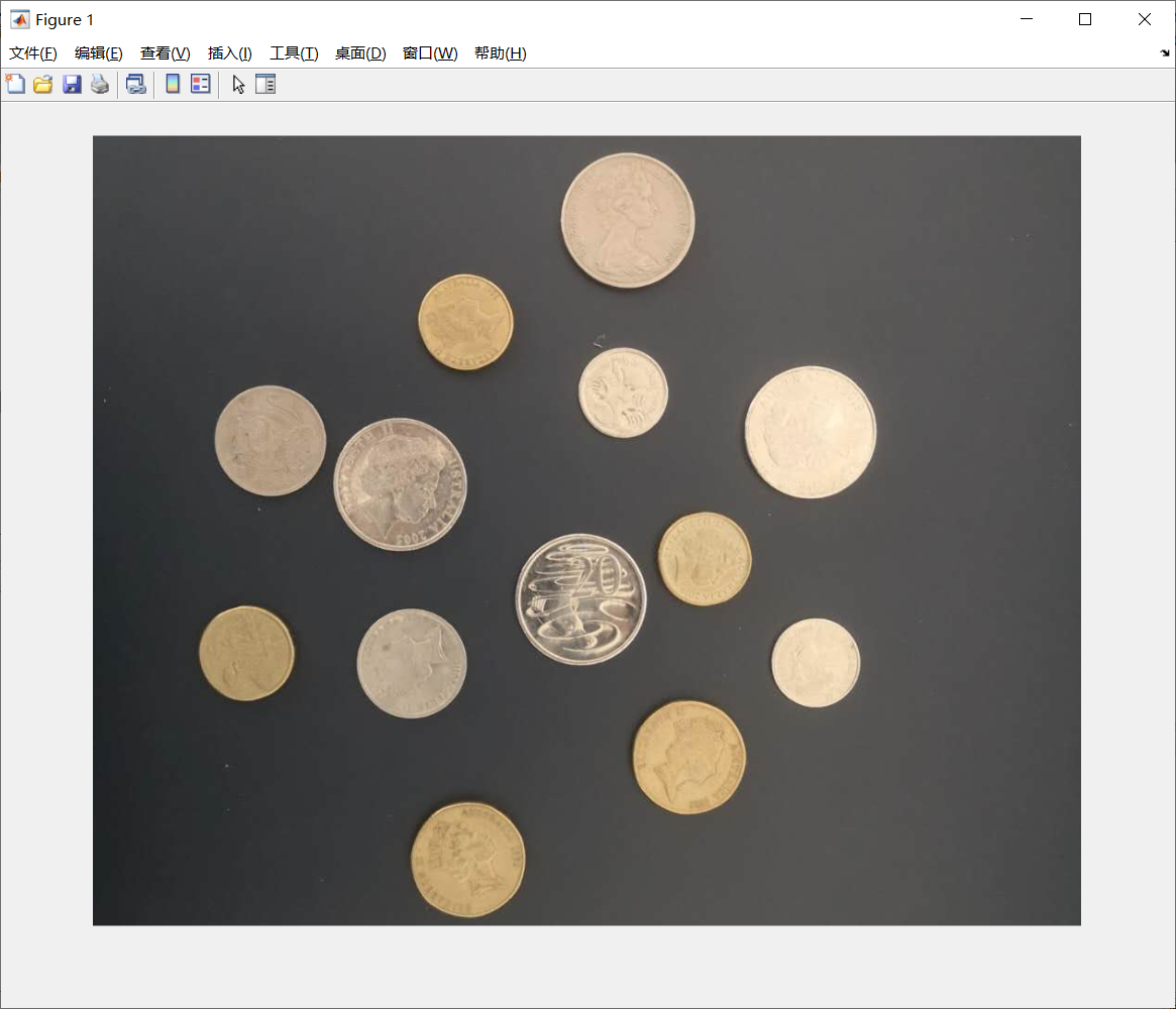
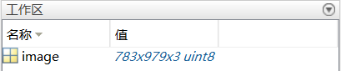
After reading, a three-dimensional matrix is obtained. 783 and 979 represent the width and length of the picture respectively, and 3 represents three channels R, G and B (three primary colors, all color pictures).

Next, convert the color image into gray image:

grayImage = rgb2gray(image);
imshow(grayImage);

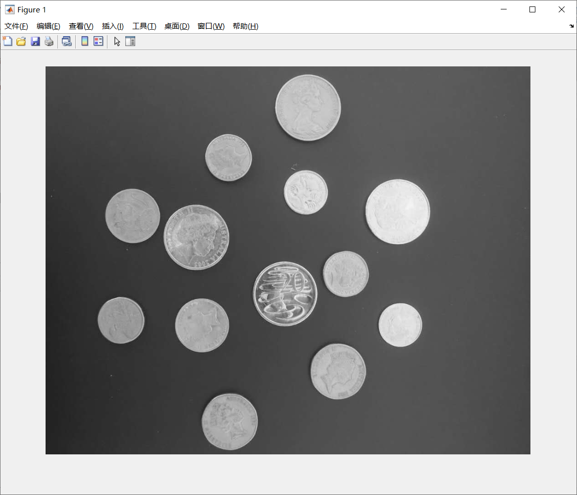
A new two-dimensional matrix is obtained. 783 and 979 represent the width and length of the picture respectively. At this time, there is no color channel.

Now use the picture properties tool to view the brightness value of picture pixels:

imtool(grayImage);

Select Inspect pixel values in the menu bar of the generated graphics window to view the brightness of each pixel, where 0 represents pure black and 255 represents pure white. From the analysis of the brightness value, it is found that the brightness of the coin is about in the range of more than 100. Write the following code:

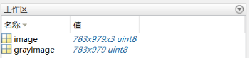
bwImage = grayImage > 100;
imshow(bwImage);

bwImage is a two-dimensional logical matrix. Logic 0 represents pure black and logic 1 represents pure white. Therefore, this line of code enables pixels with brightness greater than 100 to become pure white, and pixels with brightness less than or equal to 100 to become pure black. But now there are two kinds of defects (noise) in black-and-white pictures. The first is the residual black spots in the white circle, and the second is the white spots in the black area.

%Remove black noise
bwImage = imfill(bwImage,"hole");
imshow(bwImage);

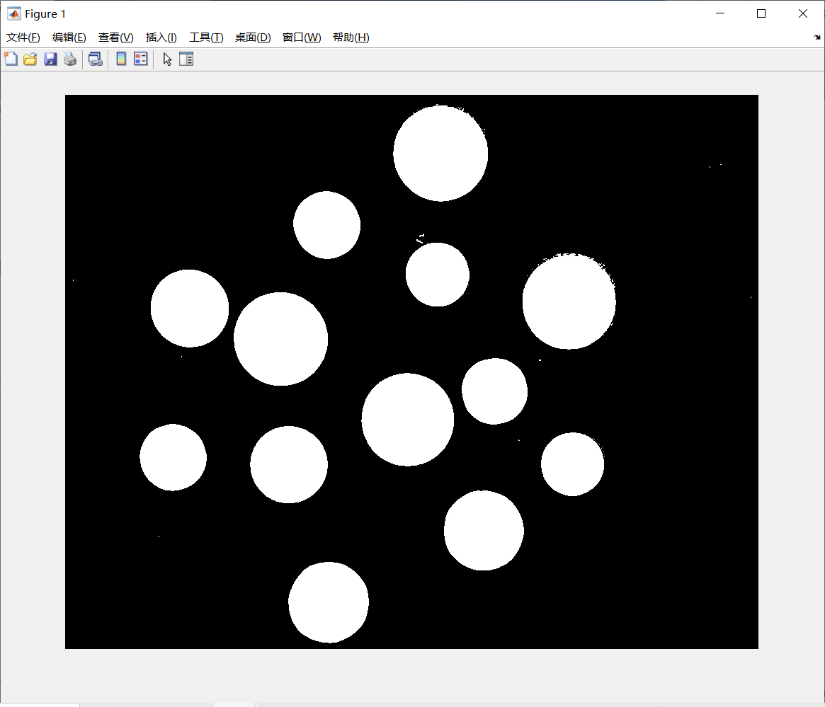
%Remove white noise
SE = strel('disk',5); %Set corrosion radius
bwImage = imerode(bwImage,SE); %corrosion
imshow(bwImage);

The corresponding to corrosion is called expansion: imdilate, but in this case, the effect of corrosion is better than expansion. Let's take a look at the effect of expansion:

SE = strel('disk',5);
bwImage = imdilate(bwImage,SE);
imshow(bwImage);

Next, count the number of coins:

[L,num] = bwlabel(bwImage); %return bwImage Number of connected regions in num in

The complete code is as follows:

clc;clear;
image = imread("coins.png");
grayImage = rgb2gray(image);
bwImage = grayImage > 100;
bwImage = imfill(bwImage,"hole");
SE = strel('disk',5);
bwImage = imerode(bwImage,SE);
[L,num] = bwlabel(bwImage);
disp(num); %13

(12.2) Mona Lisa's cat

This section introduces an encryption and anti-counterfeiting technology - "steganography".
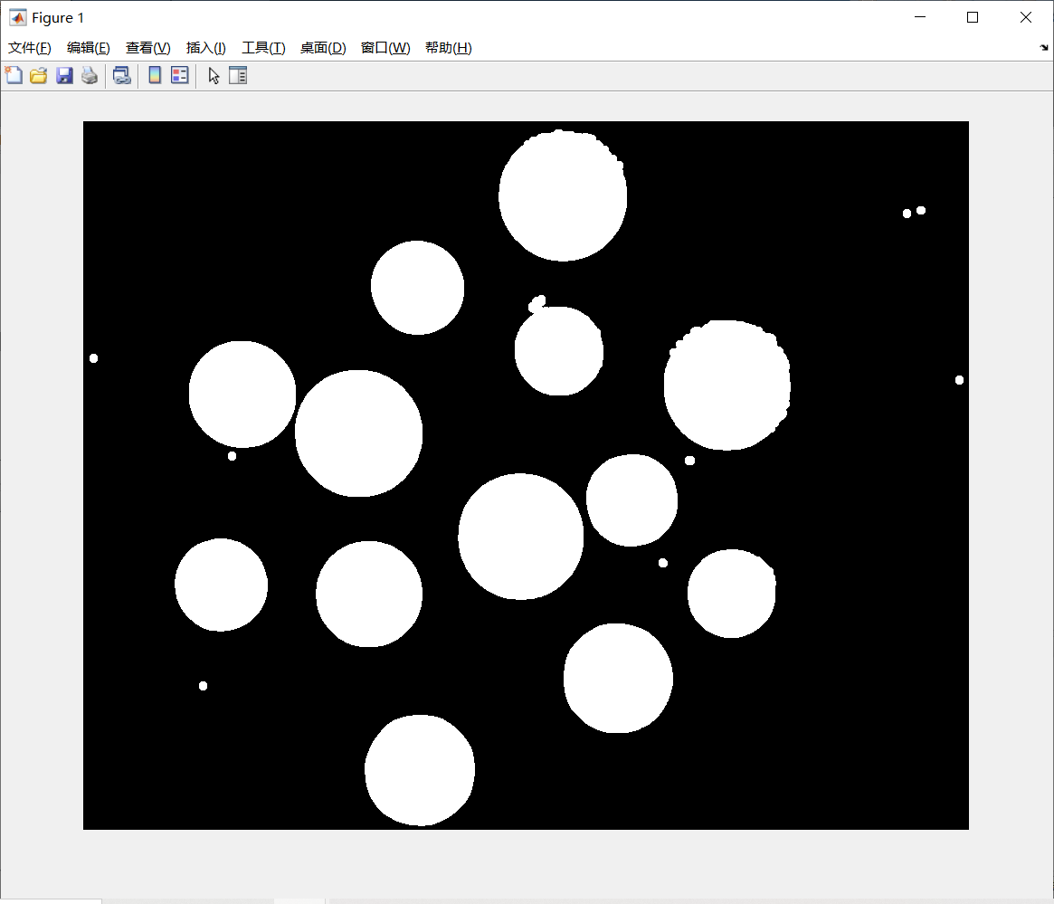
This example is to hide the picture of a cat (cat.png) into the picture of the Mona Lisa (Mona Lisa. PNG) through the superposition of pixel brightness values:

   as we have known before, the brightness value of the pixels in the gray image is between 0 and 255. 0 represents pure black and 255 represents pure white. The human naked eye cannot distinguish the brightness corresponding to the two adjacent brightness values (for example, 145 and 146, it can even be said that it is difficult to distinguish between more than 10 and more than 20 human eyes). Therefore, you can set all the single digits of the brightness value of each pixel of a picture to 0 (there is no change to the naked eye), divide the brightness value of another picture into 0 to 9, and then overlay the two pictures to hide one picture into another (but there will be a little slight distortion if you separate the picture).

%Image fusion
clc;clear;
monalisa = imread("monalisa.png");
grayMonalisa = rgb2gray(monalisa);
grayMonalisa = idivide(grayMonalisa,10)*10; %take monalisa.png The luminance single digit of the pixel becomes 0
cat = imread("cat.png");
grayCat = rgb2gray(cat);
[h,w] = size(grayMonalisa);
grayCat = imresize(grayCat,[h,w]); %take cat.png The size of is converted to and monalisa.png Consistent size
grayCat = grayCat * (9 / 255); %take cat.png The brightness of pixels is compressed to the range of 0 to 9
grayImage = grayMonalisa + grayCat; %Image fusion
imshow(grayImage); %As shown in Figure 12.2.1
imwrite(grayImage,"monalisa_cat_gray.png"); %output.png file

%Picture separation
clc;clear;
grayImage = imread("monalisa_cat_gray.png");
monalisa = idivide(grayImage,10)*10;
cat = grayImage - monalisa;
cat = cat * (255 / 9);
subplot(121);
imshow(monalisa);
subplot(122);
imshow(cat);

Based on the above principles, we can do a steganography of RGB graph:

%Fusion function
function [image] = encode(image1,image2)
    image1 = idivide(image1,10)*10;
    [h,w] = size(image1);
    image2 = imresize(image2,[h,w]);
    image2 = image2 * (9 / 255); 
    image = image1 + image2;
end

%Separation function
function [image1,image2] = decode(image)
    image1 = idivide(image,10)*10;
    image2 = image - image1;
    image2 = image2 * (255 / 9);
end

%RGB Image fusion
clc;clear;
Monalisa = imread("monalisa.png");
Cat = imread("cat.png");
MonalisaRed = Monalisa(:,:,1);
MonalisaGreen = Monalisa(:,:,2);
MonalisaBlue = Monalisa(:,:,3);
CatRed = Cat(:,:,1);
CatGreen = Cat(:,:,2);
CatBlue = Cat(:,:,3);
redImage = encode(MonalisaRed,CatRed);
greenImage = encode(MonalisaGreen,CatGreen);
blueImage = encode(MonalisaBlue,CatBlue);
image = cat(3,redImage,greenImage,blueImage); %Composite 3D matrix
imshow(image);
imwrite(image,"monalisa_cat.png");

%RGB Picture separation
clc;clear;
image = imread("monalisa_cat.png");
redImage = image(:,:,1);
greenImage = image(:,:,2);
blueImage = image(:,:,3);
[MonalisaRed,CatRed] = decode(redImage);
[MonalisaGreen,CatGreen] = decode(greenImage);
[MonalisaBlue,CatBlue] = decode(blueImage);
Monalisa = cat(3,MonalisaRed,MonalisaGreen,MonalisaBlue);
Cat = cat(3,CatRed,CatGreen,CatBlue);
subplot(121);
imshow(Monalisa);
subplot(122);
imshow(Cat);

ginseng Test Endowment material come source Reference sources Reference sources

1. Scientific computing and MATLAB language Liu Weiguo Cai Xuhui Lugley He Xiaoxian China University MOOC
2. MATLAB software and basic mathematics experiment Li Changqin Zhu Xu Wang Yongmao Ji Wanxin Xi'an Jiaotong University Press
3. MATLAB R2018a complete self-study all-in-one Liu Hao Han Jing Electronic Industry Press
4. MATLAB engineering and scientific drawing Zhou Bo Xue Shifeng Tsinghua University Press
5. Matlab tutorial - image processing (Lesson 1) The first moon lights lanterns https://www.bilibili.com.
6. Matlab tutorial - image processing (lesson 2: where is meow) The first moon lights lanterns https://www.bilibili.com.
7. MATLAB from entry to baldness Goodall https://www.bilibili.com.
8. Experimental course of automatic control principle Giant forest warehouse Xi'an Jiaotong University Press

Bo passenger create do : A i d e n   L e e Blog creation: Aiden\ Lee Blog creation: Aiden Lee
Special statement: the article is for learning reference only. Please indicate the source for reprint. Embezzlement is strictly prohibited!