1. Design purpose
Start making an interesting sound effect processing system to see if you can complete the gradual amplification and attenuation of sound, see if you can make some changes to your sound (become shrill or rough), and see what methods to change the sound playback speed. Through this course design, deepen the understanding of the theory of filter design.
2. Design requirements
1. Master DFT spectrum analysis method;
2. Master the design methods of IIR and FIR filters;
3. Master the analysis method of signal passing through linear system;
4. Be familiar with the use of MATLAB digital signal processing tools;
5. Understand the relevant knowledge of music processing.
3. Design content
3.1 voice signal acquisition
Use the recorder under Windows or other recording software to record a voice or a piece of music. Within 5s, save it as * WAV file. Then, under the Matlab software platform, use the function wavread or audioread to sample the speech signal, and remember the sampling frequency and sampling points.

[x,Fs]=audioread('E:\Course design of digital signal processing\titlttwo.wav'); 
% sound(x,Fs);
N=length(x);
n=(0:N-1);
X=fft(x); %Fourier transform
f=n/N*Fs; %Convert points to frequencies
figure(1);
subplot(2,1,1);
plot(n,x); %Draw the original sound signal
subplot(2,1,2);
plot(f,abs(X)); %Draw the amplitude spectrum of the original sound signal

3.2 design digital filter
The design index of the filter is determined according to the spectrum characteristics of the speech signal; The speech signal is processed by low-pass, high pass, band-pass and band stop filters respectively. IIR or FIR can be selected to playback the output signal, draw the time-domain waveform and spectrum, and analyze the changes before and after filtering. In MATLAB, the function sound can play back the sound. Its calling format: sound(x,fs,bits).
Reference design parameters of digital filter:
Performance index of low-pass filter: fb = 1000 Hz, fs = 1200 Hz, As = 100 dB, Ap = 1 dB
Performance index of high pass filter: fs = 4800 Hz, fb = 5000 Hz, As = 100 dB, Ap = 1 dB
Performance index of band-pass filter: fb1 = 1200 Hz, fb2 = 3000 Hz, fs1 = 1000 Hz, fs2 = 3200 Hz, As = 100 dB, Ap = 1 dB.
This time, we choose IIR filter (Butterworth filter, elliptical filter) and FIR filter (Kaiser window, etc.) to filter the speech signal, compare the clarity and tone of the filtered speech signal, and select the appropriate filter for filtering.
3.2.1 low pass filter
① IIR digital filter
Design of Butterworth low pass filter

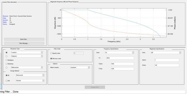
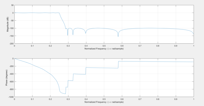
Design of elliptic low-pass filter

fp1=1000;fs1=1200; %Low pass filter passband cutoff frequency 1000 Hz And stopband cutoff frequency 1200 Hz
wp1=2*fp1/fs; ws1=2*fs1/fs;%%Calculate filter boundary frequency (about pi (normalized)
rp=1;as=100;
[N1,wp1]=ellipord(wp1,ws1,rp,as); %Calculate the order of the filter and the passband boundary frequency
[B,A]=ellip(N1,rp,as,wp1); %Calculate the filter system function coefficient vector B Sum vector A
y1=filter(B,A,x); %Filter the speech signal
% Low pass filter drawing part%
figure(2);
freqz(B,A);

② FIR digital filter
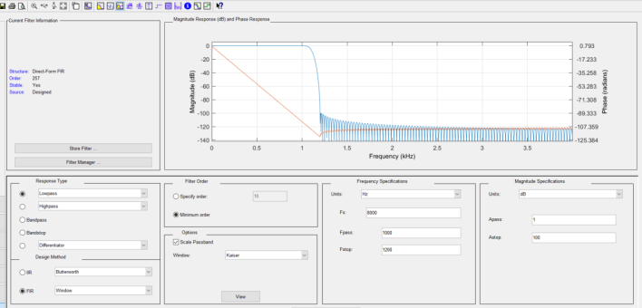
Design of Kaiser window low-pass filter

3.2.2 high pass filter
① IIR digital filter
Design Butterworth high pass filter
...
Design of elliptic high pass filter

fp2=2400;fs2=2500; %High pass filter passband cutoff frequency 2400 Hz And stopband cutoff frequency 2500 Hz
wp2=2*fp2/fs; ws2=2*fs2/fs;%Calculate the filter boundary frequency (about pi (normalized)
rp=1;as=100;
[N2,wp2]=ellipord(wp2,ws2,rp,as);
[B2,A2]=ellip(N2,rp,as,wp2,'high'); %Calculate the system function coefficient of high pass filter
y2=filter(B2,A2,x); 
% Drawing part of high pass filter%
figure(4);
freqz(B2,A2);

② FIR digital filter
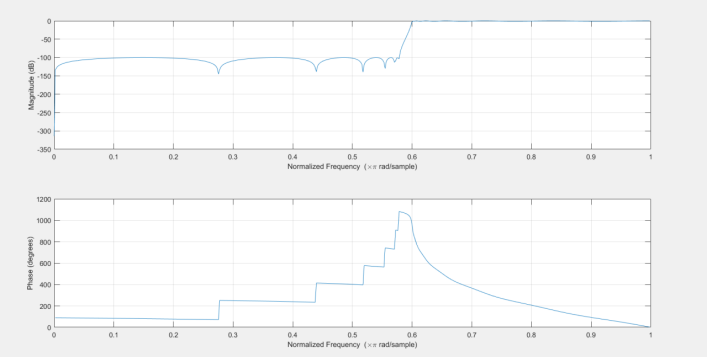
Kaiser window design high pass filter
...
3.2.3 band pass filter
① IIR digital filter
Design of Butterworth bandpass filter
...
Design of elliptic bandpass filter

fp3=[1200,3000];fs3=[1000,3200];  %Bandpass filter
wp3=2*fp3/fs; ws3=2*fs3/fs;
rp=1;as=100;
[N3,wp3]=ellipord(wp3,ws3,rp,as); %Calculate the order and passband boundary frequency of elliptic bandpass analog filter
[B3,A3]=ellip(N3,rp,as,wp3); %Calculate the function coefficients of bandpass filter and analog filter system
y3=filter(B3,A3,x); %Filter software implementation
% Drawing part of band-pass filter%
figure(6);
freqz(B3,A3);

② FIR digital filter
Kaiser window design bandpass filter
...
3.3 realize the functions of slow recording and fast playback and fast recording and slow playback
Voice variable speed without tone change refers to keeping the tone and semantics unchanged and speaking faster or slower. That is, the fundamental frequency value is almost constant, corresponding to the constant tone; The whole time process is compressed or expanded, and the number of glottic cycles decreases or increases, that is, the vocal tract movement rate changes, and the speech speed also changes. From the perspective of speech generation model, that is, the excitation and system maintain almost the same state as the original pronunciation, but the duration is longer or shorter than the original.
The principle of fast and slow playback is to play a speech sequence containing more or less information than the original sound in a long time. Take the 2-speed fast playback as an example, that is, the original 2-time voice sequence is played in the unit time. The principle here is to increase the sampling interval during playback. Then the points collected in the unit time actually contain the signals collected from the 2-length sequence (in fact, this is the lossy compression of a voice sequence). Although this will cause information loss, However, as long as the Nyquist sampling law is satisfied, the speech signal will not be distorted, so it is feasible under certain conditions.
When playing a voice sequence, you can change the sampling frequency. However, the speech signal must be processed step by step in drawing.
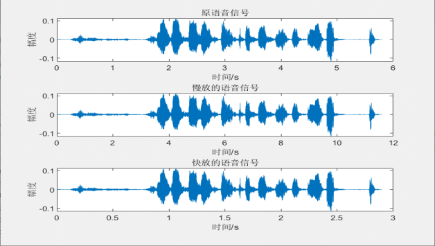
Take the fast playback as an example. If the fast playback multiple is 2, the original 10s long signal can be played within 5s, and the voice tone will become higher.

%Fast recording and slow playback
w1=0.5;
% sound(x,w1*Fs);
%Slow recording and fast playback
w2=2;
% sound(x,w2*Fs);

3.4 improvement
3.4.1 rewind
B = the array B returned by flip (A) has the same size as A, but the element order has been reversed. The reordered dimensions in B depend on the shape of A:
If A is A vector, flip(A) reverses the element order along the length of the vector.
If A is A matrix, flip(A) reverses the order of each column element.
If A is an N-dimensional array, flip(A) will operate on the first dimension where the size of A is not equal to 1.

%Audio playback
[x,Fs]=audioread('E:\Course design of digital signal processing\titlttwo.wav'); 
x1=flip(x);
sound(x1,Fs); 

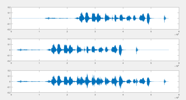
3.4.2 mixing
When sound reaches the audience in a closed space, it includes several parts: direct sound, early reflection and reverberation. The early reflection consists of the basic delay and attenuation of several spatially adjacent direct sounds, while the reverberation consists of dense echoes. The above multiple echo filter cannot provide natural sound reverberation. From its amplitude frequency characteristics, its amplitude response is not constant for all frequencies, and the listening effect is not satisfactory. Secondly, too few echoes per second will cause the vibration of synthetic sound. It takes about 1000 echoes per second to generate reflected sound without vibration.

%%%%%%%%Same signal reverberation
figure(6)
[y,Fs]=audioread('E:\Course design of digital signal processing\titlttwo.wav');
y=y(:,1);                               
%Infinite echo reverberator
a=0.5;%a Take less than or equal to 1
R=5000;                   %The higher the filter order setting, the more obvious the echo
Bz=[zeros(0,R-1),1];
Az=[1,zeros(1,R-1),-a];
y4=filter(Bz,Az,y);
subplot(3,1,1);
plot(f,y4);

%Multiple echo reverberator
N=5;
R=5000;
Bz1=[1,zeros(1,R-1),-0.5^N];
Az1=[1,zeros(1,R-1),-0.5];
y5=filter(Bz1,Az1,y);
subplot(3,1,2);
plot(f,y5);
%All pass structure reverberator
R=5000;
Bz2=[0,zeros(1,R-1),1];
Az2=[1,zeros(1,R-1),a];
y6=filter(Bz2,Az2,y);
subplot(3,1,3);
plot(f,y6);
%sound(y4);
%sound(y5);
%sound(y6);

%%%%%%%%Reverberation of two different sound signals
figure(7)
[x2,Fs]=audioread('E:\Course design of digital signal processing\di.wav'); 
m=max(size(x,1),size(x2,1));%Determine the maximum number of rows
n=max(size(x,2),size(x2,2));%Determine the maximum number of columns
xx1=zeros(m,n);
xx2=zeros(m,n);
xx1(1:size(x,1),1:size(x,2))=x; %extend x
xx2(1:size(x2,1),1:size(x2,2))=x2; %extend x2
c=1*xx1+50*xx2;
plot(f,c);
% sound(c);

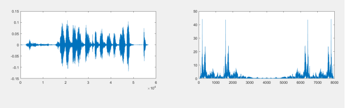
3.4.3 echo
The echo is the superposition of the original sound after the delay attenuation of the original sound. The sound signal is stored in the form of matrix in matlab.

%%%%%%%%echo
z1=[zeros(10000,1);x];%Sound delay
x1=[x;zeros(10000,1)];%Make the original sound length equal to that after delay
z=x1*0.8+z1;
figure(5);
plot(z);
% sound(z,Fs);

3.4.4 sound change
The changes of pitch period, fundamental frequency and formant frequency are mainly considered in gender sound change.

%Girls to boys
[xmen,Fs]=audioread('E:\Course design of digital signal processing\titlttwo.wav'); 
Xmen=fft(xmen);
L=length(Xmen);
temp=Xmen;
N=100;
out=vertcat(0.1*temp(1:3*N),1.2*temp(1:L),0.1*temp(1:100*N));
Ymen=1*real(ifft(out));
% sound(Ymen);
Nmen=length(Ymen);
nmen=(0:Nmen-1);
T=1/Fs;
f=nmen/Nmen*Fs; %Convert points to frequencies
subplot(2,2,1);
plot(nmen,Ymen); %Draw the sound signal after changing male voice
subplot(2,2,2);
plot(f,abs(fft(Ymen)));

%%%%%%Girls become children's voices
[xchild,Fs]=audioread('E:\Course design of digital signal processing\titlttwo.wav'); 
Xchild=fft(xchild);
L=length(Xchild);
temp=Xchild;
N=400;
out=vertcat(0.3*temp(1:N),2.5*temp(1:L),0.3*temp(1:N));
Ychild=1*real(ifft(out));
%sound(Ychild);

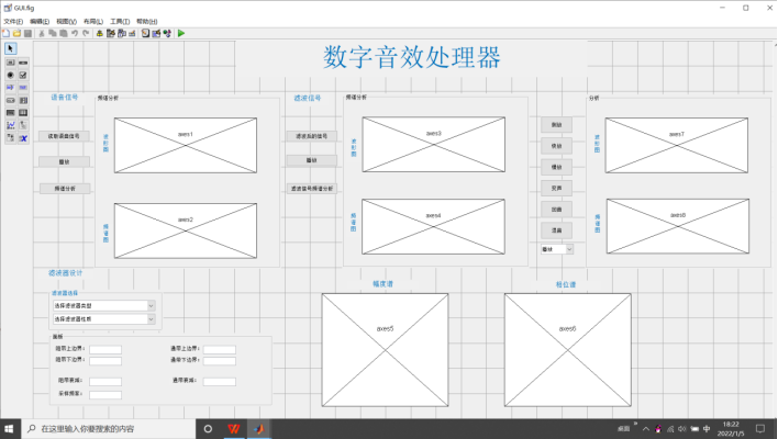
3.5 GUI interface design
In MATLAB, GUI is a graphical window containing many objects, and provides a convenient and efficient integrated development environment GUIDE for GUI development. GUIDE is mainly an interface design tool set. Matlab integrates all GUI support controls in this environment, and provides the setting method of interface appearance, properties and behavior response mode. GUIDE saves the designed GUI in a FIG file and generates an M file framework at the same time.
The page design of digital sound effect processor is carried out through the buttons and pop-up menus in the GUI navigation bar.
The interface is shown in the figure below:

After compiling the controls, we can write programs for these controls. Put the mouse on the key to be written, right-click and click callback. It will jump to the callback function of the key and write under this function.
After running, generate M file and digital sound processor as shown in the figure.

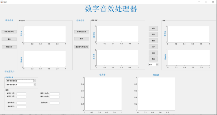
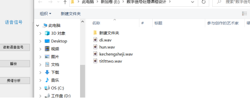
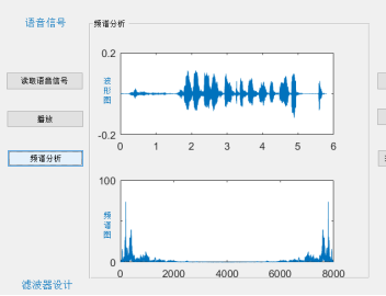
Click read voice signal, select wav file to read and display waveform diagram.

Click the play button to play the read voice signal, and click spectrum analysis to display the spectrum diagram of the read voice signal.

The filter design part can select the type and nature of the filter through the drop-down menu.

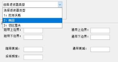
After selection, fill in the editable text box below according to the design parameters. You can fill in different parameters, observe the amplitude spectrum and phase spectrum of the generated filter, and select an appropriate filter to filter the speech signal.
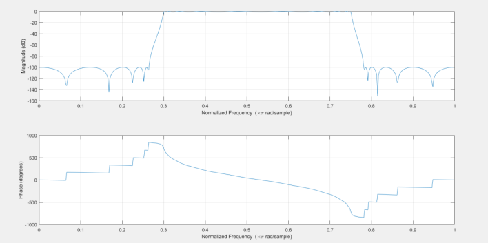
Take elliptic high pass filter as an example:
Select fs = 2400 Hz, fb = 2500 Hz, As = 100 dB, Ap = 1 dB.

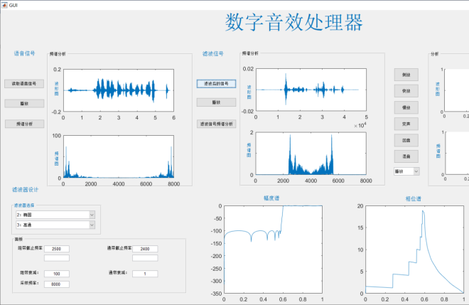
We can observe the amplitude spectrum and phase spectrum of the generated filter. At first, there are some problems in the horizontal axis coordinates on this figure, not the normalized frequency. I tried to use the axis function to constrain the abscissa, but there was a problem with the graph. After the teacher pointed out this problem, I went back to consult the data and found that the abscissa should be specified. After specifying the abscissa as w/pi, I got the normalized frequency.
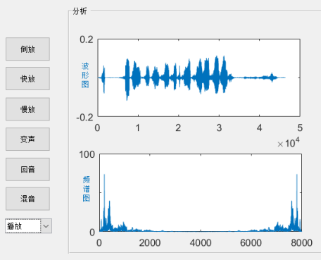
Other functions are realized through buttons:
Press the button to observe the waveform and spectrum of the processed speech signal and analyze it.
You can play while pressing the button, or you can play selectively and multiple times through the drop-down menu.

4. Result analysis
4.1 speech signal spectrum analysis

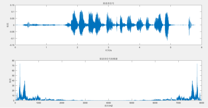
The collected language signal is about 5s, and the frequency is concentrated in 100-1000HZ.
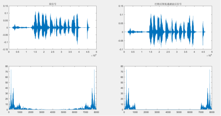
4.2 filter the signal with a filter
%%Butterworth low pass filter
Hd1=ditong;
yfilter1=filter(Hd1,x);
figure(2);
subplot(2,2,1);
plot(n,x); % Draw the original sound signal
title('original signal ');
subplot(2,2,3);
plot(f,abs(X)); % Draw the amplitude spectrum of the original sound signal
subplot(2,2,2);
plot(yfilter1);
title('butterworth low pass filtered signal ');
Y1=abs(fft(yfilter1));
subplot(2,2,4);
plot(f,Y1);

... others
...
4.3 slow recording and fast playback and fast recording and slow playback

4.4 improvement
%%Inverted

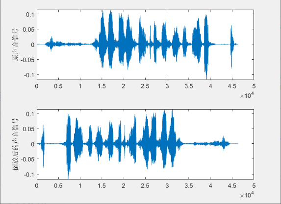
After rewinding, I can't hear what the original voice says, and the tone changes a little.
%%Mix

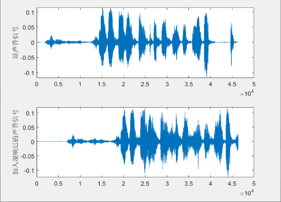
If you mix the same voice signal, you can hear countless voice signals playing at different times. If different voice signals are mixed, you can hear the two voice signals superimposed together and played at the same time.
%%Echo

The first figure is the waveform of the voice signal after a period of time delay. The second figure is after the original voice signal is zeroed. When they are superimposed together, you can hear the echo effect of the voice signal. The echo was clear.
%%Sound change

When a female voice becomes a male voice, the voice becomes lower because the fundamental frequency and formant frequency change.
5. Summary
...

reference
[1] Gao Xiquan, Ding Yumei. Digital signal processing (Third Edition). Xi'an University of Electronic Science and Technology Press. two thousand and ten
[2] Edited by Zhang Defeng. MATLAB digital signal processing and application. Tsinghua University Press. two thousand and ten
[3] Roey Lzhaki, translated by Lei Wei Mixing guide People's Posts and Telecommunications Publishing House two thousand and eighteen
[4] Cong Yuliang, edited by Wang Zhihong. Digital signal processing principle and its MATLAB implementation. Electronic Industry Press. two thousand and nine
[5] Fang Weiwei, Hao Ying Audio processing system based on MATLAB GUI [J] Modern computer, 2021,27 (25): 115-120
[6] Edited by Cao Ge. matlab tutorial and training. China Machine Press. two thousand and twenty