Batch Normalization
Forward
The first small problem is that let's realize the forward propagation of BN layer. For a batch of samples, calculate their mean and variance, then standardize the data, and finally don't forget to add a certain offset. The code is as follows:
def batchnorm_forward(x, gamma, beta, bn_param):
    """
    Forward pass for batch normalization.

    During training the sample mean and (uncorrected) sample variance are
    computed from minibatch statistics and used to normalize the incoming data.
    During training we also keep an exponentially decaying running mean of the
    mean and variance of each feature, and these averages are used to normalize
    data at test-time.

    At each timestep we update the running averages for mean and variance using
    an exponential decay based on the momentum parameter:

    running_mean = momentum * running_mean + (1 - momentum) * sample_mean
    running_var = momentum * running_var + (1 - momentum) * sample_var

    Note that the batch normalization paper suggests a different test-time
    behavior: they compute sample mean and variance for each feature using a
    large number of training images rather than using a running average. For
    this implementation we have chosen to use running averages instead since
    they do not require an additional estimation step; the torch7
    implementation of batch normalization also uses running averages.

    Input:
    - x: Data of shape (N, D)
    - gamma: Scale parameter of shape (D,)
    - beta: Shift paremeter of shape (D,)
    - bn_param: Dictionary with the following keys:
      - mode: 'train' or 'test'; required
      - eps: Constant for numeric stability
      - momentum: Constant for running mean / variance.
      - running_mean: Array of shape (D,) giving running mean of features
      - running_var Array of shape (D,) giving running variance of features

    Returns a tuple of:
    - out: of shape (N, D)
    - cache: A tuple of values needed in the backward pass
    """
    mode = bn_param['mode']
    eps = bn_param.get('eps', 1e-5)
    momentum = bn_param.get('momentum', 0.9)

    N, D = x.shape
    running_mean = bn_param.get('running_mean', np.zeros(D, dtype=x.dtype))
    running_var = bn_param.get('running_var', np.zeros(D, dtype=x.dtype))

    out, cache = None, None
    if mode == 'train':
        #######################################################################
        # TODO: Implement the training-time forward pass for batch norm.      #
        # Use minibatch statistics to compute the mean and variance, use      #
        # these statistics to normalize the incoming data, and scale and      #
        # shift the normalized data using gamma and beta.                     #
        #                                                                     #
        # You should store the output in the variable out. Any intermediates  #
        # that you need for the backward pass should be stored in the cache   #
        # variable.                                                           #
        #                                                                     #
        # You should also use your computed sample mean and variance together #
        # with the momentum variable to update the running mean and running   #
        # variance, storing your result in the running_mean and running_var   #
        # variables.                                                          #
        #                                                                     #
        # Note that though you should be keeping track of the running         #
        # variance, you should normalize the data based on the standard       #
        # deviation (square root of variance) instead!                        #
        # Referencing the original paper (https://arxiv.org/abs/1502.03167)   #
        # might prove to be helpful.                                          #
        #######################################################################
        sample_mean = np.mean(x, axis = 0)
        sample_var = np.var(x, axis = 0)
        x_after = (x - sample_mean) / np.sqrt(sample_var + eps)
        out = gamma * x_after + beta
        running_mean = momentum * running_mean + (1 - momentum) * sample_mean
        running_var = momentum * running_var + (1 - momentum) * sample_var
        inv_var = 1.0 / np.sqrt(sample_var + eps)
        cache = (x, x_after, gamma, inv_var, sample_mean)
        #######################################################################
        #                           END OF YOUR CODE                          #
        #######################################################################
    elif mode == 'test':
        #######################################################################
        # TODO: Implement the test-time forward pass for batch normalization. #
        # Use the running mean and variance to normalize the incoming data,   #
        # then scale and shift the normalized data using gamma and beta.      #
        # Store the result in the out variable.                               #
        #######################################################################
        x_after = (x - running_mean) / np.sqrt(running_var + eps)
        out = gamma * x_after + beta
        #######################################################################
        #                          END OF YOUR CODE                           #
        #######################################################################
    else:
        raise ValueError('Invalid forward batchnorm mode "%s"' % mode)

    # Store the updated running means back into bn_param
    bn_param['running_mean'] = running_mean
    bn_param['running_var'] = running_var

    return out, cache
Note that in test, we do BN to standardize a fixed mean and variance.
Backward
The next problem is to realize the back propagation of BN layer, which has puzzled me for most of the time. At the beginning, what I thought was too simple, which led to the calculation error of dx all the time. The reason is that I didn't understand the real meaning of back propagation before. In order to carry out back propagation, the best way is to draw a calculation chart, decompose the complex expressions into simple operations, and then calculate the derivative step by step, so that the upstream gradient will continue to accumulate and flow to the downstream. It is highly recommended to understand the calculation of dx expression in BN layer This article , it's really the great God in the great God. I read his article and finally got the expression of dx right. The code is as follows:
def batchnorm_backward(dout, cache):
    """
    Backward pass for batch normalization.

    For this implementation, you should write out a computation graph for
    batch normalization on paper and propagate gradients backward through
    intermediate nodes.

    Inputs:
    - dout: Upstream derivatives, of shape (N, D)
    - cache: Variable of intermediates from batchnorm_forward.

    Returns a tuple of:
    - dx: Gradient with respect to inputs x, of shape (N, D)
    - dgamma: Gradient with respect to scale parameter gamma, of shape (D,)
    - dbeta: Gradient with respect to shift parameter beta, of shape (D,)
    """
    dx, dgamma, dbeta = None, None, None
    ###########################################################################
    # TODO: Implement the backward pass for batch normalization. Store the    #
    # results in the dx, dgamma, and dbeta variables.                         #
    # Referencing the original paper (https://arxiv.org/abs/1502.03167)       #
    # might prove to be helpful.                                              #
    ###########################################################################
    x, x_after, gamma, inv_var, sample_mean = cache
    N, D = dout.shape[0], dout.shape[1]
    dgamma = np.ones(N).dot(dout * x_after)
    dbeta = np.ones(N).dot(dout)
    ########## dx ###########
    dx1 = dout * gamma * inv_var
    dx2 = np.ones(N).dot(dout * gamma * (x - sample_mean))
    dx2 *= -(inv_var ** 2)
    dx2 *= 0.5 * inv_var
    dx2 = (1.0 / N) * np.ones((N, D)) * dx2
    dx2 *= 2 * (x - sample_mean)
    dx = dx1 + dx2
    dx1 = dx
    dx2 = -np.ones(N).dot(dx)
    dx2 = (1.0 / N) * np.ones((N, D)) * dx2
    dx = dx1 + dx2
    #########################
    ###########################################################################
    #                             END OF YOUR CODE                            #
    ###########################################################################

    return dx, dgamma, dbeta
The gradients of beta and gamma are easy to calculate. According to the unified method of attention dimension mentioned in the previous article, we get the expression. According to the calculation chart drawn by Da Shen, when we calculate DX, we need to multiply and calculate gradients step by step. Specifically, each step is a common derivation operation. However, we need to make sure that the gradients we get are dimensionally unified with the current variables after each node. Compared with the writing method of np.sum(mat, axis = 0), I am more accustomed to using np.ones(N).dot(mat), which The principle that we are ensuring the unity of dimensions can be better reflected in the example. I only use dx1 and dx2 here to show the iterative process, which is not very clear. The clear writing method must see the article of the great God, which really makes me praise!
After the implementation of the basic back propagation, the task asks us to deduce the formula of the back propagation of the BN layer on the paper and write out a long string of calculation expressions directly. This place is also a key point. The main steps of the derivation can be summarized with this figure Here)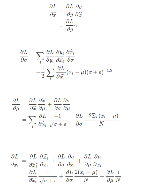
After this writing, I think I have a deeper understanding of reverse communication. It's really not good to just look at it without hands. If you want to really understand reverse communication, you must push your hands to knock the code again! The implementation code is as follows, 17 times faster than the original (I don't know how fat four It's slow to see others...)
Since we need to add layer_norm next, we will not be able to load the code for the time being, and finally we will load it together.
Next, the assignment shows us the differences between the full connected network trained by adding BN layer and not adding BN layer, such as high accuracy, fast convergence, not strict requirements for weight initialization, etc. To sum up, BN is good. We must add BN! At the same time, another important conclusion is that generally speaking, the more samples BN layer contains, the better the final effect is. It's easy to understand. Because the more samples, the more accurate the statistical results are, the better the effect is naturally. But for the test, because the mean value and square deviation of BN are fixed, it has nothing to do with our batch size.
Layer Normalization
The next problem is to realize Layer Normalization, which is actually to standardize the feature dimension. What do you mean? We take a transposition of the original input and turn it into a matrix of (D, N) size, then do the same Batch Normalization operation, and finally turn the result back. The corresponding back propagation is the same. First, we take a transpose of dx_after, and then for the previous operation, change the corresponding n into D. after the operation is completed, we can transpose DX back successfully. This is the charm of linear algebra! (although I probably know it's right to write like this, I haven't turned my mind completely and am ready to supplement my knowledge of linear algebra qwq)
def layernorm_forward(x, gamma, beta, ln_param):
    """
    Forward pass for layer normalization.

    During both training and test-time, the incoming data is normalized per data-point,
    before being scaled by gamma and beta parameters identical to that of batch normalization.

    Note that in contrast to batch normalization, the behavior during train and test-time for
    layer normalization are identical, and we do not need to keep track of running averages
    of any sort.

    Input:
    - x: Data of shape (N, D)
    - gamma: Scale parameter of shape (D,)
    - beta: Shift paremeter of shape (D,)
    - ln_param: Dictionary with the following keys:
        - eps: Constant for numeric stability

    Returns a tuple of:
    - out: of shape (N, D)
    - cache: A tuple of values needed in the backward pass
    """
    out, cache = None, None
    eps = ln_param.get('eps', 1e-5)
    ###########################################################################
    # TODO: Implement the training-time forward pass for layer norm.          #
    # Normalize the incoming data, and scale and  shift the normalized data   #
    #  using gamma and beta.                                                  #
    # HINT: this can be done by slightly modifying your training-time         #
    # implementation of  batch normalization, and inserting a line or two of  #
    # well-placed code. In particular, can you think of any matrix            #
    # transformations you could perform, that would enable you to copy over   #
    # the batch norm code and leave it almost unchanged?                      #
    ###########################################################################
    x = x.T
    sample_mean = np.mean(x, axis = 0)
    sample_var = np.var(x, axis = 0)
    x_after = (x - sample_mean) / np.sqrt(sample_var + eps)
    x_after = x_after.T
    out = gamma * x_after + beta
    inv_var = 1.0 / np.sqrt(sample_var + eps)
    cache = (x, x_after, gamma, beta, inv_var, sample_mean)
    ###########################################################################
    #                             END OF YOUR CODE                            #
    ###########################################################################
    return out, cache


def layernorm_backward(dout, cache):
    """
    Backward pass for layer normalization.

    For this implementation, you can heavily rely on the work you've done already
    for batch normalization.

    Inputs:
    - dout: Upstream derivatives, of shape (N, D)
    - cache: Variable of intermediates from layernorm_forward.

    Returns a tuple of:
    - dx: Gradient with respect to inputs x, of shape (N, D)
    - dgamma: Gradient with respect to scale parameter gamma, of shape (D,)
    - dbeta: Gradient with respect to shift parameter beta, of shape (D,)
    """
    dx, dgamma, dbeta = None, None, None
    ###########################################################################
    # TODO: Implement the backward pass for layer norm.                       #
    #                                                                         #
    # HINT: this can be done by slightly modifying your training-time         #
    # implementation of batch normalization. The hints to the forward pass    #
    # still apply!                                                            #
    ###########################################################################
    x, x_after, gamma, beta, inv_var, sample_mean = cache
    N, D = dout.shape[0], dout.shape[1]
    dgamma = np.ones(N).dot(dout * x_after)
    dbeta = np.ones(N).dot(dout)
    dx_after = dout * gamma
    dx_after = dx_after.T
    dvar = np.ones(D).dot(dx_after * (-0.5) * (x - sample_mean) * np.power(inv_var, 3))
    dmean = np.ones(D).dot(dx_after * (-inv_var)) + np.ones(D).dot(dvar * (-2.0 / D) * (x - sample_mean))
    dx = dx_after * inv_var + dvar * 2.0 * (x - sample_mean) / D + dmean / D
    dx = dx.T
    ###########################################################################
    #                             END OF YOUR CODE                            #
    ###########################################################################
    return dx, dgamma, dbeta
Next, add the code of BN and LN to the full connection network:
class FullyConnectedNet(object):
    """
    A fully-connected neural network with an arbitrary number of hidden layers,
    ReLU nonlinearities, and a softmax loss function. This will also implement
    dropout and batch/layer normalization as options. For a network with L layers,
    the architecture will be

    {affine - [batch/layer norm] - relu - [dropout]} x (L - 1) - affine - softmax

    where batch/layer normalization and dropout are optional, and the {...} block is
    repeated L - 1 times.

    Similar to the TwoLayerNet above, learnable parameters are stored in the
    self.params dictionary and will be learned using the Solver class.
    """

    def __init__(self, hidden_dims, input_dim=3*32*32, num_classes=10,
                 dropout=1, normalization=None, reg=0.0,
                 weight_scale=1e-2, dtype=np.float32, seed=None):
        """
        Initialize a new FullyConnectedNet.

        Inputs:
        - hidden_dims: A list of integers giving the size of each hidden layer.
        - input_dim: An integer giving the size of the input.
        - num_classes: An integer giving the number of classes to classify.
        - dropout: Scalar between 0 and 1 giving dropout strength. If dropout=1 then
          the network should not use dropout at all.
        - normalization: What type of normalization the network should use. Valid values
          are "batchnorm", "layernorm", or None for no normalization (the default).
        - reg: Scalar giving L2 regularization strength.
        - weight_scale: Scalar giving the standard deviation for random
          initialization of the weights.
        - dtype: A numpy datatype object; all computations will be performed using
          this datatype. float32 is faster but less accurate, so you should use
          float64 for numeric gradient checking.
        - seed: If not None, then pass this random seed to the dropout layers. This
          will make the dropout layers deteriminstic so we can gradient check the
          model.
        """
        self.normalization = normalization
        self.use_dropout = dropout != 1
        self.reg = reg
        self.num_layers = 1 + len(hidden_dims)
        self.dtype = dtype
        self.params = {}

        ############################################################################
        # TODO: Initialize the parameters of the network, storing all values in    #
        # the self.params dictionary. Store weights and biases for the first layer #
        # in W1 and b1; for the second layer use W2 and b2, etc. Weights should be #
        # initialized from a normal distribution centered at 0 with standard       #
        # deviation equal to weight_scale. Biases should be initialized to zero.   #
        #                                                                          #
        # When using batch normalization, store scale and shift parameters for the #
        # first layer in gamma1 and beta1; for the second layer use gamma2 and     #
        # beta2, etc. Scale parameters should be initialized to ones and shift     #
        # parameters should be initialized to zeros.                               #
        ############################################################################
        self.params['W1'] = weight_scale * np.random.randn(input_dim, hidden_dims[0])
        self.params['b1'] = np.zeros(hidden_dims[0])
        if self.normalization is not None:
            self.params['gamma1'] = np.ones(hidden_dims[0])
            self.params['beta1'] = np.zeros(hidden_dims[0])
        for i in range(1, self.num_layers - 1):
            self.params['W' + str(i + 1)] = weight_scale * np.random.randn(hidden_dims[i - 1], hidden_dims[i])
            self.params['b' + str(i + 1)] = np.zeros(hidden_dims[i])
            if self.normalization is not None:
                self.params['gamma' + str(i + 1)] = np.ones(hidden_dims[i])
                self.params['beta' + str(i + 1)] = np.zeros(hidden_dims[i])
        self.params['W' + str(self.num_layers)] = weight_scale * np.random.randn(hidden_dims[self.num_layers - 2], num_classes)
        self.params['b' + str(self.num_layers)] = np.zeros(num_classes)
        ############################################################################
        #                             END OF YOUR CODE                             #
        ############################################################################

        # When using dropout we need to pass a dropout_param dictionary to each
        # dropout layer so that the layer knows the dropout probability and the mode
        # (train / test). You can pass the same dropout_param to each dropout layer.
        self.dropout_param = {}
        if self.use_dropout:
            self.dropout_param = {'mode': 'train', 'p': dropout}
            if seed is not None:
                self.dropout_param['seed'] = seed

        # With batch normalization we need to keep track of running means and
        # variances, so we need to pass a special bn_param object to each batch
        # normalization layer. You should pass self.bn_params[0] to the forward pass
        # of the first batch normalization layer, self.bn_params[1] to the forward
        # pass of the second batch normalization layer, etc.
        self.bn_params = []
        if self.normalization=='batchnorm':
            self.bn_params = [{'mode': 'train'} for i in range(self.num_layers - 1)]
        if self.normalization=='layernorm':
            self.bn_params = [{} for i in range(self.num_layers - 1)]

        # Cast all parameters to the correct datatype
        for k, v in self.params.items():
            self.params[k] = v.astype(dtype)


    def loss(self, X, y=None):
        """
        Compute loss and gradient for the fully-connected net.

        Input / output: Same as TwoLayerNet above.
        """
        X = X.astype(self.dtype)
        mode = 'test' if y is None else 'train'

        # Set train/test mode for batchnorm params and dropout param since they
        # behave differently during training and testing.
        if self.use_dropout:
            self.dropout_param['mode'] = mode
        if self.normalization=='batchnorm':
            for bn_param in self.bn_params:
                bn_param['mode'] = mode
        scores = None
        ############################################################################
        # TODO: Implement the forward pass for the fully-connected net, computing  #
        # the class scores for X and storing them in the scores variable.          #
        #                                                                          #
        # When using dropout, you'll need to pass self.dropout_param to each       #
        # dropout forward pass.                                                    #
        #                                                                          #
        # When using batch normalization, you'll need to pass self.bn_params[0] to #
        # the forward pass for the first batch normalization layer, pass           #
        # self.bn_params[1] to the forward pass for the second batch normalization #
        # layer, etc.                                                              #
        ############################################################################
        out = X
        affine_cache, relu_cache, bn_cache, ly_cache = [], [], [], []
        for i in range(1, self.num_layers):
            out, cache = affine_forward(out, self.params['W' + str(i)], self.params['b' + str(i)])
            affine_cache.append(cache)
            if self.normalization == 'batchnorm':
                out, cache = batchnorm_forward(out, self.params['gamma' + str(i)], self.params['beta' + str(i)], self.bn_params[i - 1])
                bn_cache.append(cache)
            elif self.normalization == 'layernorm':
                out, cache = layernorm_forward(out, self.params['gamma' + str(i)], self.params['beta' + str(i)], self.bn_params[i - 1])
                ly_cache.append(cache)
            out, cache = relu_forward(out)
            relu_cache.append(cache)
        out, cache = affine_forward(out, self.params['W' + str(self.num_layers)], self.params['b' + str(self.num_layers)])
        affine_cache.append(cache)
        scores = out
        ############################################################################
        #                             END OF YOUR CODE                             #
        ############################################################################

        # If test mode return early
        if mode == 'test':
            return scores

        loss, grads = 0.0, {}
        ############################################################################
        # TODO: Implement the backward pass for the fully-connected net. Store the #
        # loss in the loss variable and gradients in the grads dictionary. Compute #
        # data loss using softmax, and make sure that grads[k] holds the gradients #
        # for self.params[k]. Don't forget to add L2 regularization!               #
        #                                                                          #
        # When using batch/layer normalization, you don't need to regularize the scale   #
        # and shift parameters.                                                    #
        #                                                                          #
        # NOTE: To ensure that your implementation matches ours and you pass the   #
        # automated tests, make sure that your L2 regularization includes a factor #
        # of 0.5 to simplify the expression for the gradient.                      #
        ############################################################################
        loss, dout = softmax_loss(scores, y)
        reg_loss = 0
        for i in range(1, self.num_layers + 1):
            reg_loss += np.sum(self.params['W' + str(i)] * self.params['W' + str(i)])
        reg_loss *= (0.5 * self.reg)
        loss += reg_loss
        dx, grads['W' + str(self.num_layers)], grads['b' + str(self.num_layers)] = affine_backward(dout, affine_cache[self.num_layers - 1])
        grads['W' + str(self.num_layers)] += self.reg * self.params['W' + str(self.num_layers)]
        for i in range(self.num_layers - 1, 0, -1):
            dx = relu_backward(dx, relu_cache[i - 1])
            if self.normalization == 'batchnorm':
                dx, grads['gamma' + str(i)], grads['beta' + str(i)] = batchnorm_backward_alt(dx, bn_cache[i - 1])
            elif self.normalization == 'layernorm':
                dx, grads['gamma' + str(i)], grads['beta' + str(i)] = layernorm_backward(dx, ly_cache[i - 1])
            dx, grads['W' + str(i)], grads['b' + str(i)] = affine_backward(dx, affine_cache[i - 1])
            grads['W' + str(i)] += self.reg * self.params['W' + str(i)]
            grads['b' + str(i)] += self.reg * self.params['b' + str(i)]
        ############################################################################
        #                             END OF YOUR CODE                             #
        ############################################################################

        return loss, grads
A simple little problem
When is layer normalization likely to not work well, and why?
1.Using it in a very deep network
2.Having a very small dimension of features
3.Having a high regularization term
The answer is 2. Because Layer Normalization is essentially Batch Normalization after transposition, the smaller the feature dimension is, the smaller the batch size when BN is.
Well, that's the end of the second question. I think the second question gives me a deeper understanding of the specific derivation of computational graphs and back propagation. Although I don't need to write these derivations after applying the framework, it's very important to understand the principle behind them. Especially, a series of fancy operations of matrices make me realize the lack of my knowledge of linear algebra, Ready to go to see the line to replace qwq
Welcome criticism and correction~

