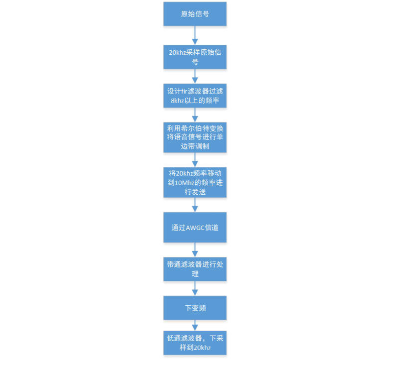
Overall flow chart of FIR filter design

This design uses fir filter to filter the speech signal. This simulation design uses matlab as the simulation platform and the signal of matlab as the original speech signal to simulate the filter. The flow chart is shown as follows:

General design flow chart

The first thing to design is the fir filter. According to the theoretical form of the fir filter, the fir filter (finite length impulse response) is an all zero filter, and its mathematical realization form is as follows:

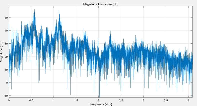
The two most important characteristics of the filter are linear phase characteristic and amplitude characteristic. The frequency characteristic curve of the original signal is shown in Figure 1.1. Through cubic spline interpolation, the sampling rate of the speech signal is increased to 20Khz. The spectrum diagram after sampling is shown in Figure 1.2.

Figure 1.1: spectrum diagram of original signal

Figure 1.2: spectrum diagram of increasing sampling to 20khz

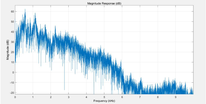
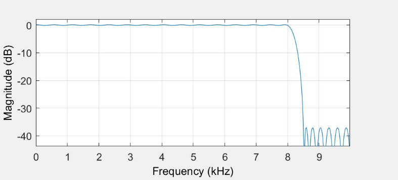
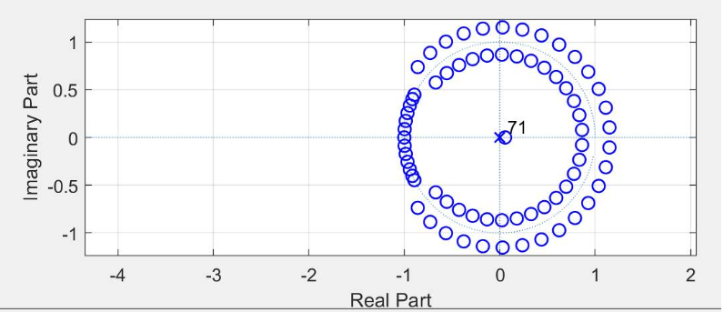
After observing Figure 1.2, it can be found that the energy of the signal is concentrated in the low-frequency part. In order to reduce the useless high-frequency components, the fir low-pass filter is designed to filter them out. In this design, equal ripple is sampled to complete the design of low-pass filter. The design tool uses the filter tool FADTOOL of MATLAB. FAD can quickly verify and design the filter according to the user's parameters. According to the spectrum diagram in Figure 1.2, determine the fp = 8khz and fs = 8.5khz of the designed low-pass filter. The spectrum diagram of the designed filter is shown in Figure 1.3, its order is 71, and the zero pole distribution of the unit circle is shown in Figure 1.4

Figure 1.3: spectrum diagram of low-pass filter

Figure 1.4: zero pole distribution of FIR filter

After the speech signal passes through the low-pass filter, its spectral response is shown in Figure 1.5.

Figure 1.5 speech signal spectrum through low-pass signal

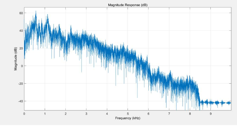
It can be clearly seen that the spectrum of the signal greater than 8khz is filtered.

After filtering, Hilbert filtering is used to transform the double sideband signal of speech signal into single sideband signal to reduce the use of communication bandwidth. Here, the Hilbert filter \ (\ frac{1}{\pi t} \) of matlab is designed to filter the spectrum of the signal, as shown in Fig. 1.6. The single sideband frequency is changed by Hilbert change, as shown in Fig. 1.7.

Figure 1.6 bilateral spectrum of speech signal

Figure 1.7 single side spectrum of speech signal

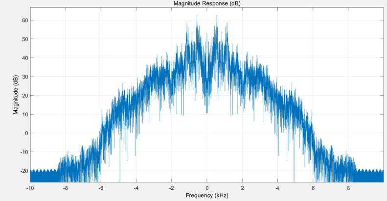
Since the signal needs to be transmitted, for example, the frequency is increased, and the sampling rate of 20khz is converted to that of 10M. Generally, phased sampling is used to increase the sampling rate by 500 times. Increasing the sampling rate each time is equivalent to extending the spectrum. In order to ensure the shape of the spectrum, filters with fir settings of 0.2 and 0.25 are used for processing. Figure 1.8 shows the spectrum of 5 times upsampling.

Figure 1.8 spectrum diagram of voice signal after up sampling 5 times

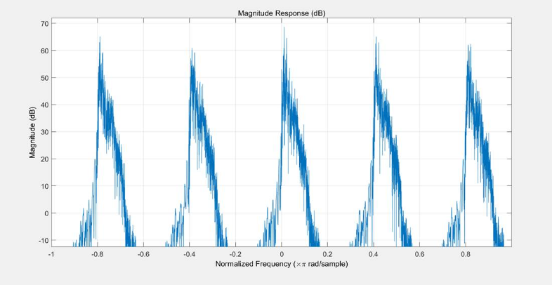
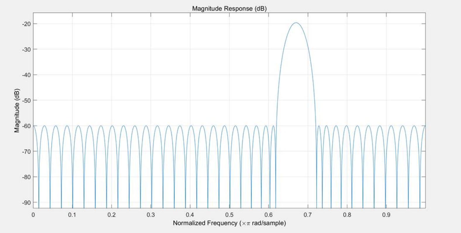
Therefore, the filter is filtered with a cut-off frequency of 0.2, and the frequency response of the filter is shown in Figure 1.9.

Fig. 1.9 spectrum diagram of low-pass filter with cut-off frequency of 0.2 Figure 1.10 shows the spectrum of a low-pass filter with a cut-off frequency of 0.25


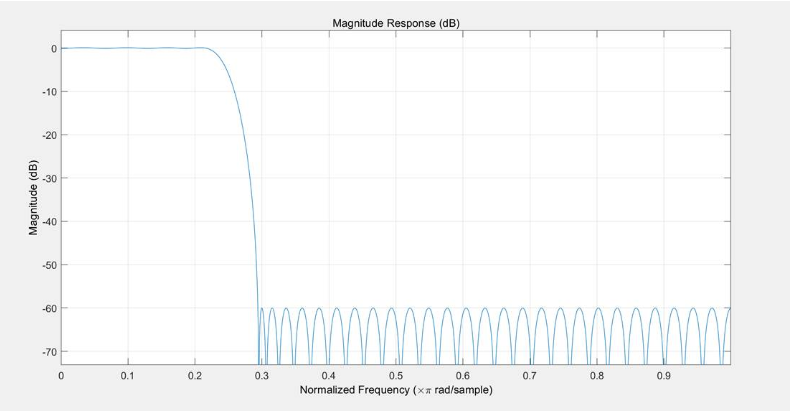
Fig. 1.10 spectrum diagram of low-pass filter with cut-off frequency of 0.2

When the voice signal is upsample d by 500 times, its spectrum diagram is shown in Figure 1.11 below.

Figure 1.11: spectrum of voice waveform after upsample

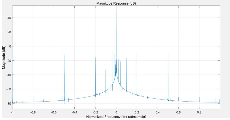
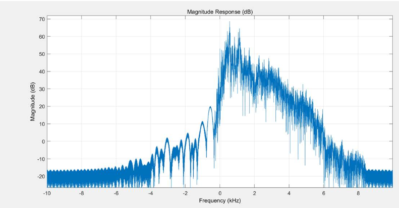
Finally, the frequency of the voice signal is moved so that the signal can be transmitted. The spectrum diagram of speech signal after spectrum transfer is shown in Figure 1.12.

Figure 1.12: spectrum pattern of voice signal after moving through the spectrum

The design of speech signal through AWGN channel is equivalent to adding a Gaussian white noise to the spectrum of speech signal. The spectrum of Gaussian white noise is shown in Figure 1.12.

Fig. 1.12 spectrum of Gaussian white noise

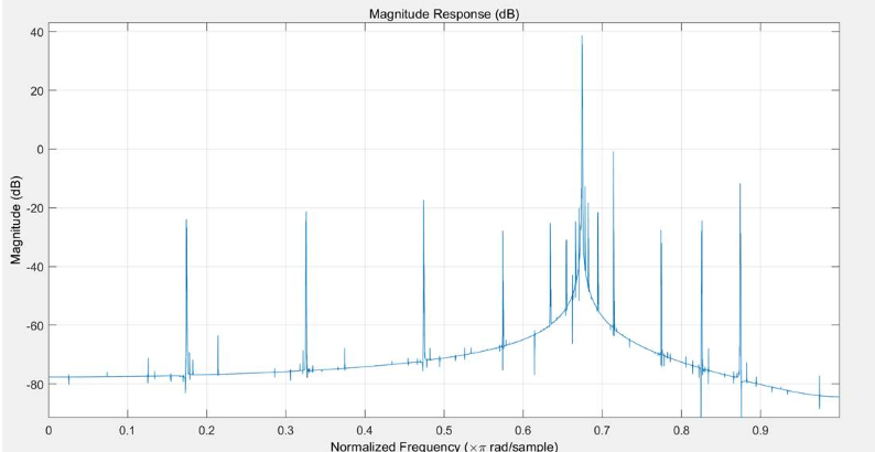
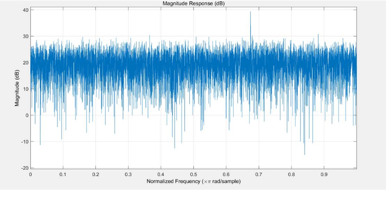
Summarizing the above process, the voice signal is sampled and increased to 10M to meet the transmission conditions, and Gaussian white noise is used to simulate the signal noise impact caused by the channel in the process. At this time, to receive the original signal and demodulate the original signal, the receiver must have a band-pass filter to filter out the speech signal and discard the useless noise signal. According to the spectrum in Fig. 1.11, the band-pass of the band-pass filter is 0.6-0.75. The minimum ripple design is selected by using the FAD of MATLAB to obtain the normalized coefficient matrix of the band-pass filter, and its frequency response is shown in Fig. 1.13.

Figure 1.13: frequency response graph of bandpass filter

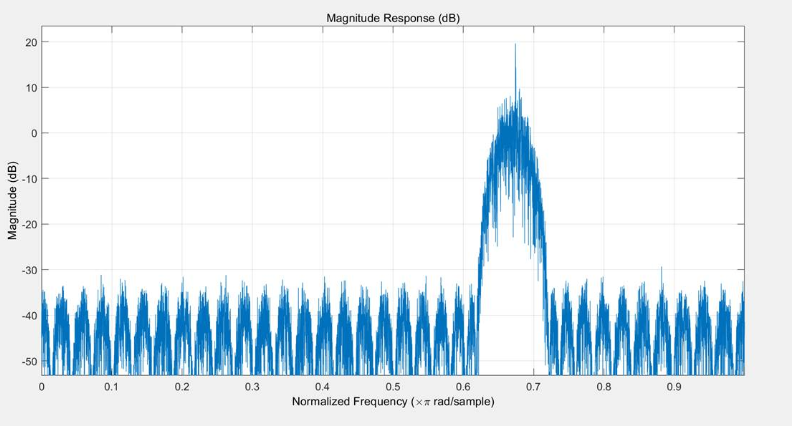
The speech spectrum of the received signal after band-pass filtering is shown in Figure 1.14.

Figure 1.14: frequency response graph of voice signal passing through band-pass filter

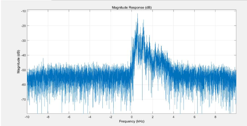
The received voice signal is subjected to dowmsample (lower side frequency processing). Similarly, the down conversion is 500, and the process is opposite to the up conversion. Finally, the spectrum of the heard speech signal is shown in Figure 1.15.

By listening to the original signal and the received signal through the sound function of matlab, it is found that the voice of the signal is basically the same, so the communication of voice signal and the simulation of filter through this scheme are successful and feasible.

clear all
close all
clc
%% 
load handel
h = fvtool(y);
set(h, 'Fs', Fs);
sound(y, Fs);
pause(10)

% The first step is to increase the voice sampling rate to 20 KHz
T = (length(y)-1) / Fs;
Y = interp1( [0:1/Fs:T], y, [0:1/20e3:T], 'spline');
h = fvtool(Y);
set(h, 'Fs', 20e3);
sound(Y, 20e3);
pause(10)


% Connect signal 8 KHz Filter out the above part,For details of design method, see fdatool
voiceCoef = [-0.00331567291687537,0.00302323989662157,0.00236335999433444,-0.000249895806141854,0.00324405325416548,-0.00268876267273492,0.00360296141490172,-0.00230710811907060,0.00100163740863659,0.00152582296780255,-0.00388560018913911,0.00604697828734485,-0.00697045946214204,0.00639302318173106,-0.00395271528961120,-2.33446800352772e-05,0.00492259451573453,-0.00964894184901816,0.0129924208661240,-0.0137833678820759,0.0112660249790563,-0.00531183793788302,-0.00339120178077228,0.0133543120529965,-0.0224465890588835,0.0282360533532409,-0.0284263495578446,0.0213310613052760,-0.00627693990578004,-0.0161429286985805,0.0440352410987295,-0.0744109723115057,0.103606516887248,-0.127851104964425,0.143880717742118,0.850515547752914,0.143880717742118,-0.127851104964425,0.103606516887248,-0.0744109723115057,0.0440352410987295,-0.0161429286985805,-0.00627693990578004,0.0213310613052760,-0.0284263495578446,0.0282360533532409,-0.0224465890588835,0.0133543120529965,-0.00339120178077228,-0.00531183793788302,0.0112660249790563,-0.0137833678820759,0.0129924208661240,-0.00964894184901816,0.00492259451573453,-2.33446800352772e-05,-0.00395271528961120,0.00639302318173106,-0.00697045946214204,0.00604697828734485,-0.00388560018913911,0.00152582296780255,0.00100163740863659,-0.00230710811907060,0.00360296141490172,-0.00268876267273492,0.00324405325416548,-0.000249895806141854,0.00236335999433444,0.00302323989662157,-0.00331567291687537];
dispFilterResponse(voiceCoef, 1/20e3, '');
voice = filter(voiceCoef, 1, Y);
h = fvtool(voice);
set(h, 'Fs', 20e3);
sound(voice, 20e3);
pause(10)

% Realization of single sideband by filtering method,Hilbert filter needs to be designed, 1/(pi*t)
d = fdesign.hilbert('N,TW',200, 0.1);
Hd = design(d,'equiripple','SystemObject',true);
Realvoice = circshift(voice, 100);
Imagvoice = filter(Hd.Numerator, 1, voice);

h = fvtool(Realvoice);
set(h, 'FrequencyRange','[-pi, pi)');
set(h, 'Fs', 20e3);
h = fvtool(Realvoice + 1i*Imagvoice);
set(h, 'Fs', 20e3);


Basebandvoice = Realvoice + 1i*Imagvoice;


% 20K->10M The sampling rate needs to be increased by 500 times. There are 500 stages here = 5 * 5 * 5 * 4，The cut-off frequencies to be designed are 0.2 And 0.25 Two kinds of filters
x5Coef = [0.00112692337568268,0.00158692025434125,0.00205896989050378,0.00197709384758320,0.00111473190427317,-0.000472447774337975,-0.00236605559284221,-0.00385845971455964,-0.00419282731353260,-0.00290235997397991,-0.000113082201514355,0.00334505346493630,0.00612323159188132,0.00682609929601474,0.00462600477070206,-0.000226559774923881,-0.00625173793228883,-0.0110992424858532,-0.0123738225850133,-0.00866846592173900,-0.000402088021268619,0.00993919626594012,0.0183840950231772,0.0208076890127266,0.0146172933092511,0.000185101945744734,-0.0185805496678055,-0.0348933246131477,-0.0409283295252545,-0.0303450353032694,-0.000682784674361512,0.0452255563608527,0.0994103424861294,0.150580752726224,0.187122188502142,0.200369871454618,0.187122188502142,0.150580752726224,0.0994103424861294,0.0452255563608527,-0.000682784674361512,-0.0303450353032694,-0.0409283295252545,-0.0348933246131477,-0.0185805496678055,0.000185101945744734,0.0146172933092511,0.0208076890127266,0.0183840950231772,0.00993919626594012,-0.000402088021268619,-0.00866846592173900,-0.0123738225850133,-0.0110992424858532,-0.00625173793228883,-0.000226559774923881,0.00462600477070206,0.00682609929601474,0.00612323159188132,0.00334505346493630,-0.000113082201514355,-0.00290235997397991,-0.00419282731353260,-0.00385845971455964,-0.00236605559284221,-0.000472447774337975,0.00111473190427317,0.00197709384758320,0.00205896989050378,0.00158692025434125,0.00112692337568268];
x4Coef = [0.000856994565694856,0.000591393177382970,-3.85351917650751e-05,-0.00130837344797337,-0.00269292916711479,-0.00331425686614336,-0.00244296037940879,-9.10921433942072e-05,0.00271899015730028,0.00432293869924751,0.00336191370561577,-0.000190182688008892,-0.00462501376328013,-0.00718415092444753,-0.00565091781262915,8.72027154765229e-06,0.00706737732439220,0.0111778371760113,0.00888277600993286,0.000135749254865209,-0.0108425521935169,-0.0173232948547436,-0.0138880550352155,-0.000292556888299184,0.0170984534611941,0.0277598485492297,0.0226701214314515,0.000423692149837658,-0.0297645353604724,-0.0505233937915195,-0.0438668534604438,-0.000511549520956627,0.0737481607287266,0.158297486795985,0.225157564979538,0.250542370102760,0.225157564979538,0.158297486795985,0.0737481607287266,-0.000511549520956627,-0.0438668534604438,-0.0505233937915195,-0.0297645353604724,0.000423692149837658,0.0226701214314515,0.0277598485492297,0.0170984534611941,-0.000292556888299184,-0.0138880550352155,-0.0173232948547436,-0.0108425521935169,0.000135749254865209,0.00888277600993286,0.0111778371760113,0.00706737732439220,8.72027154765229e-06,-0.00565091781262915,-0.00718415092444753,-0.00462501376328013,-0.000190182688008892,0.00336191370561577,0.00432293869924751,0.00271899015730028,-9.10921433942072e-05,-0.00244296037940879,-0.00331425686614336,-0.00269292916711479,-0.00130837344797337,-3.85351917650751e-05,0.000591393177382970,0.000856994565694856];

tmp = upsample(Basebandvoice, 5);
tmp = filter(x5Coef, 1, tmp);
tmp = upsample(tmp, 5);
tmp = filter(x5Coef, 1, tmp);
tmp = upsample(tmp, 5);
tmp = filter(x5Coef, 1, tmp);
tmp = upsample(tmp, 4);
tmp = filter(x4Coef, 1, tmp);
h = fvtool(tmp);
set(h, 'Fs', 10e6);

TX = tmp .* exp(1i * 2 * pi * 3.37e6 * [1:length(tmp)]/10e6);
TX = real(TX);
h = fvtool(TX);
set(h, 'Fs', 10e6);

%% after AWGN channel
RX = awgn(TX, -10, 'measured');
h = fvtool(RX);
set(h, 'Fs', 10e6);

%% Receiver
% Bandpass filtering
bandpassCoef = [-0.000220985157474574	-0.000603199022228535	0.000567700620989989	-0.000144856835556256	-0.000537413993393477	0.000811952546260190	-0.000221093885213475	-0.000818227351198006	0.00123133214160066	-0.000365497144552332	-0.00113169408536944	0.00172960562049404	-0.000556315269703292	-0.00146815254434005	0.00229154024087189	-0.000793782309906573	-0.00180607660804564	0.00288989310575587	-0.00107147573190690	-0.00212115551648486	0.00349042252209103	-0.00137783322201238	-0.00238983933967575	0.00405551842218856	-0.00169658391251432	-0.00259081022572485	0.00454537432747044	-0.00200659683781057	-0.00270824168828992	0.00492493249491361	-0.00228582462373403	-0.00273356399437629	0.00516543626532525	-0.00251194689244855	-0.00266626182302852	0.00524743941405402	-0.00266626182302852	-0.00251194689244855	0.00516543626532525	-0.00273356399437629	-0.00228582462373403	0.00492493249491361	-0.00270824168828992	-0.00200659683781057	0.00454537432747044	-0.00259081022572485	-0.00169658391251432	0.00405551842218856	-0.00238983933967575	-0.00137783322201238	0.00349042252209103	-0.00212115551648486	-0.00107147573190690	0.00288989310575587	-0.00180607660804564	-0.000793782309906573	0.00229154024087189	-0.00146815254434005	-0.000556315269703292	0.00172960562049404	-0.00113169408536944	-0.000365497144552332	0.00123133214160066	-0.000818227351198006	-0.000221093885213475	0.000811952546260190	-0.000537413993393477	-0.000144856835556256	0.000567700620989989	-0.000603199022228535	-0.000220985157474574];
tmp = filter(bandpassCoef, 1, RX);
h = fvtool(tmp);
set(h, 'Fs', 10e6);

% Down conversion
tmp = tmp .* exp(-1i * 2 * pi * 3.37e6 * [1:length(tmp)]/10e6);
h = fvtool(tmp);
set(h, 'Fs', 10e6);  % Note that there is an image, which will be removed by the filter below

% Low pass filtering, down sampling to 20 KHz
tmp = filter(x4Coef, 1, tmp);
tmp = downsample(tmp, 4);
tmp = filter(x5Coef, 1, tmp);
tmp = downsample(tmp, 5);
tmp = filter(x5Coef, 1, tmp);
tmp = downsample(tmp, 5);
tmp = filter(x5Coef, 1, tmp);
tmp = downsample(tmp, 5);

h = fvtool(tmp);
set(h, 'Fs', 20e3);

% Play music
sound(real(tmp)*1e3, 20e3);
pause(10)

%% Draw the corresponding
function y = dispFilterResponse(coef, Fs, text) 
[h1,w1]=freqz(coef,1);  
plot(w1/pi*Fs/2,20*log10(abs(h1))); 
grid;
xlabel('frequency') ;
ylabel(text) ;
end