What is target tracking: tracking a target in an image, to put it bluntly, is to track a small image in the image. Remember the concept of image and small image, so let's start.  

Mean shift principle

The principle of mean shift is to find the local optimum according to the gradient climb of probability density.

probability density

If you want to know probability density, you have to know what probability is first?

Obviously, this probability is the probability that a pixel in the image is in a small image.

So what is probability density?

We don't need to know much, because we just need probability density as a medium for judgment.

Simply remember, the area with higher probability has a higher probability density.

For example, in the above figure, the probability density in the upper right corner is greater than that in the lower left corner.

Gradient climb

What is gradient climb?

According to the above probability density knowledge, now we want to track this small image, so we must chase it from the place with low probability density to the place with high probability density (after all, the greater the probability density, the greater the probability of these pixels in the small image, the greater the probability of the small image in the image), right~

Let's use something else as an example of gradient climbing

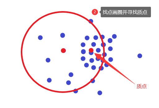
Look at the point diagram below. How to find the most concentrated position of points?

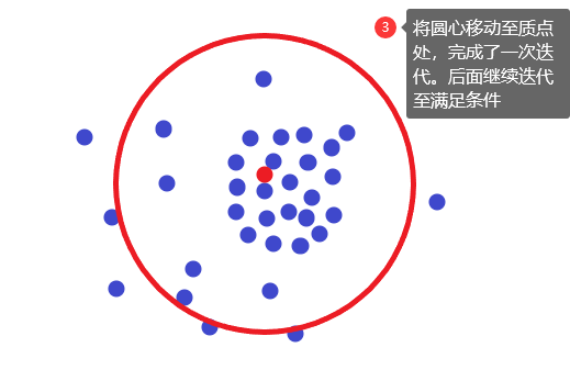
First find a point randomly, circle a circle, find the place with the most points in the circle (called a particle), and then move the center of the circle to the position of the particle, so as to complete an iteration. Finally, iterate until the center of the circle coincides with the particle or the distance between the center of the circle and the particle is at least less than a certain threshold.

Convert pixel values to probability values

After reading the above two sections, we understand that the main contradiction now is how to convert the pixel values of each pixel of the image into probability values. Once converted to the probability value, as long as the iterative gradient climb, the target tracking will be completed naturally, and all problems will be solved!

Conversion method: histogram back projection

In my opinion, the more specific point of histogram back projection should be: the pixel value of the image is back projected into the probability value according to the normalized histogram of the small image.

Use an example to illustrate:

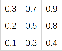
1. This is the pixel value of a part of the image:

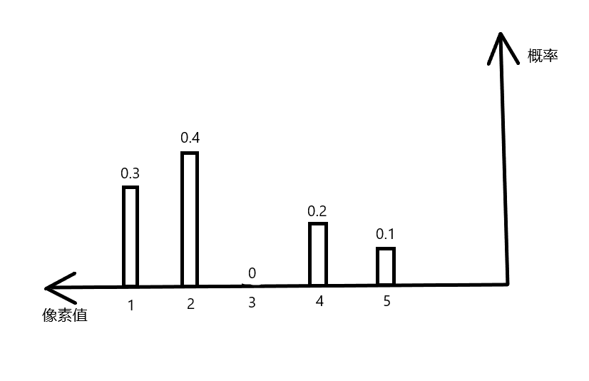
2. This is the normalized histogram of the small image:

PS: those who do not understand normalized histogram can read this article: Histogram , or just look around on csdn.

3. Then, the image part transformed according to the normalized histogram of the small image becomes:

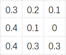
It's quite simple. That's the principle~

meanshift in OpenCv

import numpy as np
import cv2 as cv

# Read video
cap = cv.VideoCapture('car.mp4')

# Step 1: get the normalized histogram of small image
ret,frame = cap.read()
x, y, w, h = 100, 325, 100, 50
roi = frame[y:y+h, x:x+w]                                                   # ROI is a small image.
hsv_roi =  cv.cvtColor(roi, cv.COLOR_BGR2HSV)                               # Convert ROI to HSV color space
mask = cv.inRange(hsv_roi, np.array((0, 60,32)), np.array((180,255,255)))   # Remove the position where the color is too bright or too dark in the POI
roi_hist = cv.calcHist([hsv_roi],[0],mask,[180],[0,180])                    # ROI histogram
cv.normalize(roi_hist,roi_hist,0,180,cv.NORM_MINMAX)                        # ROI histogram normalization

# Set the tracking window (step 2: prerequisites)
track_window = (x, y, w, h)
# Set the termination condition, which can be 10 iterations or move at least 1 pt (the second step is the precondition)
term_crit = ( cv.TERM_CRITERIA_EPS | cv.TERM_CRITERIA_COUNT, 10, 1 )

# The second step is histogram back projection
while(1):
    ret, frame = cap.read()
    if ret == True:
        
        # Original image to HSV
        hsv = cv.cvtColor(frame, cv.COLOR_BGR2HSV)

        # Histogram back projection is performed on the basis of ROI histogram normalization
        dst = cv.calcBackProject([hsv],[0],roi_hist,[0,180],1)

        # Apply meanshift to get the new location
        ret, track_window = cv.meanShift(dst, track_window, term_crit)

        # Draw a frame on the image to track the small image
        x,y,w,h = track_window
        img = cv.rectangle(frame, (x,y), (x+w,y+h), 255,2)

        cv.namedWindow('img', 0)
        cv.imshow('img',img)
        k = cv.waitKey(30) & 0xff
        if k == 27:
            break
    else:
        break

Note: the code in the above example is converted to HSV color space, because the small image must be found according to the color characteristics, while the RGB color space needs 3 channels to indicate the color, while the HSV color space only needs a single channel (H channel) to express the color clearly.

The above is the personal learning understanding after learning. If there are errors, please point out!

Therefore, reprint is prohibited! Please send a private letter if necessary.