Radar target echo

Firstly, the composition and structure of radar target echo are introduced, and then the students have an in-depth understanding of the generation of target echo through code.

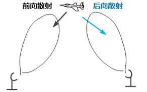
The echo received by radar can be forward scattering or backward scattering. Backscattering is usually unique to bistatic radar.
The signal received by the radar can be expressed as
  x ( t ) = S ( t ) + N ( t ) + C ( t ) + J ( t ) \ x(t) = S(t)+N(t)+C(t) +J(t)  x(t)=S(t)+N(t)+C(t)+J(t)
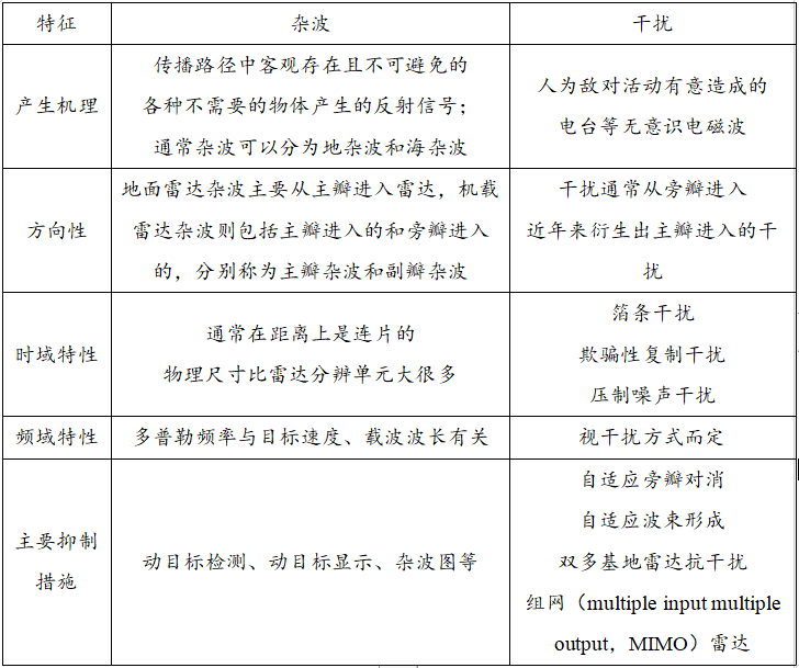
Among them, S ( t ) S(t) S(t) represents the backscattered echo of the target, N ( t ) N(t) N(t) represents noise, C ( t ) C(t) C(t) is expressed as clutter, J ( t ) J(t) J(t) indicates interference

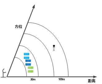
In the figure below, different colors at 30m represent the haystacks with different swings caused by wind speed. Therefore, in the distance azimuth plane, it can be seen that the haystacks should also be widened and distributed on the distance velocity plane. People are at the intersection of a distance unit and a velocity unit. Therefore, the received signal should be the sum of the scattered signal of the haystack and the human signal, i.e
  x = ∑ i J s ( t − τ i ) + s ( t − τ 0 ) \ x=\sum_{i}^Js(t-\tau_i)+s(t-\tau_0)  x=i∑J​s(t−τi​)+s(t−τ0​)
Among them, τ 0 \tau_0 τ 0 ￠ indicates the unit where the person is located, τ i \tau_i τ i ， indicates the second i i The scattering delay of i haystacks, J indicates that the swing speed of the haystack has j levels.

Radar target echo pulse compression

Here, the signal in the received signal is mainly S ( t ) S(t) S(t). Clutter and interference will be introduced in turn in subsequent meetings
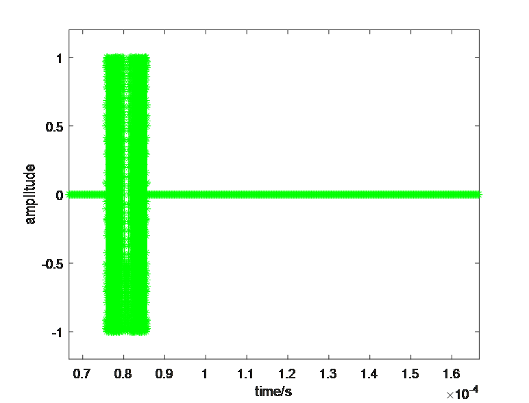
Taking LFM LFM signal as an example, the target echo expression is:

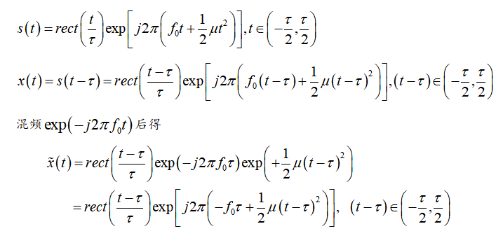
When generating echo, there are usually two methods. One is to calculate the position of the target distance, convert it into sampling points, and then move the transmitted signal directly to the position according to the sampling points. In this case, the phase of the first point of the received signal is the same as that of the first point of the transmitted signal. In fact, according to the wave propagation, When he moves from the initial position to the target position, the initial phase of the first point touching the target is not necessarily consistent with the initial phase of the transmitted signal, so the radar usually judges the time delay of the received signal through the reference crystal oscillator of the transmitted signal, and compensates the phase corresponding to the time delay, The phase of the first point of the received signal is the same as the initial phase of the transmitted signal. In the process of simulation, it is not necessary to study this problem deeply, and the received signal after mixing can be directly generated.

pulse compression

Matched filter (MF) is the filter that maximizes the output signal-to-noise ratio when the input is signal and additive white noise, which is the best filter matched with the input signal.
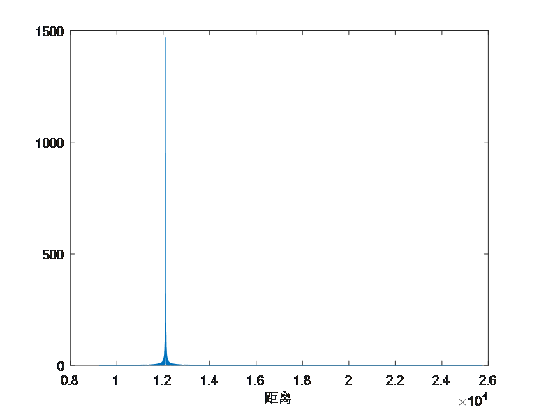
The target echo can obtain the maximum signal-to-noise ratio output through the matched filter, so as to obtain the target distance.

Simulation of radar target echo pulse compression

Target distance: 121000m
(1) Echo signal

(2) Pulse pressure results

code

// An highlighted block
clc;clear all;close all
c=3e8;          %light speed
% LFM Signal parameters
f0=10e9;
Tp=10e-6;       %Transmitted signal pulse width
B=30e6;         %Transmission signal bandwidth
mu=B/Tp;       %Frequency modulation rate
fs= 5*B;        %sampling frequency 
Tr=1e-3;        %Transmit signal pulse repetition period
Rmin = 10e3;    %Nearest distance  % Rmin = Tp/2*c;  %Theoretical detection distance 
Rmax = 25e3;    %Farthest distance  % Rmax = (Tr-Tp/2)*c;%The longest distance theoretically detected
Tstar= 2*Rmin/c;  
Tend= 2*Rmax/c;   % Tstar and Tend Respectively represents the starting time of the sampling time
%  Generation time series
t=Tstar: 1/fs: Tend-1/fs;   % Time series of sampling process
% Detection range
Rwin= linspace(Rmin, Rmax, length(t))-0.25*c*Tp;  % Remember to subtract the distance of half the pulse width
% For the specific principle, please refer to the courseware of Lecture 7 radar target echo simulation
% Parameters of a single target
R0=12.1e3 ;      %Initial distance of target
%  Generate the received signal of a single target
tao = 2*R0/c;   %  tao Represents the amount of delay of the target
td = t-tao ;
Echo = exp(j*2*pi*(-f0*tao+0.5*mu*td.^2)).*(abs(td)<Tp/2); 
figure(1), plot(t, real(Echo),'g-*');
xlabel('time/s');ylabel('amplitude'); axis([t(1) t(end) -1.2 1.2]);

t0=linspace(-Tp/2,Tp/2,Tp*fs);
ht=exp(-j*pi*mu*t0.^2);    % matched filter 
% Time domain convolution method 
y1=conv(Echo,ht);
% The output of convolution is higher than the input signal Echo1 A long pulse width, i.e Tp Therefore, when drawing later
% To increase the length of the axis
Rwin1= [Rwin max(Rwin)+1/fs*c/2*(1:round(Tp*fs)-1)];
% Frequency domain multiplication
hf=fft(ht,length(Echo));
y2=ifft(fftshift(fft(Echo).*hf));

figure,plot(Rwin1,abs(y1));
xlabel('distance')