EfficientNet learning notes

1. Thesis ideas

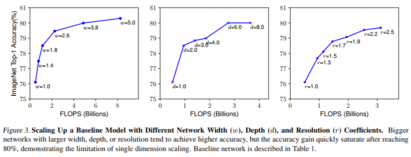
In some previous papers, some will improve the performance of the network by increasing the width of the network, that is, increasing the number of convolution cores (increasing the channels of the characteristic matrix), as shown in figure (b), and some will improve the performance of the network by increasing the depth of the network, that is, using more layer structures, as shown in figure (b) © As shown in figure (d), some will improve the performance of the network by increasing the resolution of the input network, as shown in figure (d). In this paper, the network width, the network depth and the resolution of the input network will be increased to improve the network performance, as shown in figure (e):

Based on past experience, it is not difficult to find:
(1) Increasing the depth of the network can get richer and more complex features, and can be well applied to other tasks. However, if the depth of the network is too deep, it will face the problems of gradient disappearance and difficult training.
(2) Increasing the width of the network can obtain higher fine-grained features and easier to train, but it is often difficult to learn deeper features for networks with large width and shallow depth.
(3) Increasing the image resolution of the input network can potentially obtain higher fine-grained feature templates, but for very high input resolution, the gain of accuracy will also decrease, and large-resolution images will increase the amount of calculation.

The following figure shows the statistical results obtained by adding width, depth and resolution to the benchmark efficientbet0-0 respectively. As can be seen from the figure below, it tends to be saturated when the Accuracy reaches 80%.

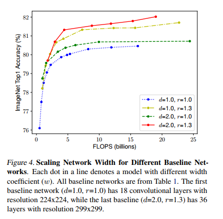
Then the author did another experiment, using different combinations of d and r, and then constantly changing the width of the network to obtain four curves as shown in the figure below. Through analysis, it can be found that under the same FLOPs, the effect of increasing d and r at the same time is the best.

The author abstracts the calculation of the whole network model:

among F i L i F_i^{L_i} FiLi ， indicates the execution of the i-th stage operation L i L_i Li times, X means S t a g e i Stage_i The characteristic matrix of Stagei, H i , W i , C i H_i,W_i,C_i Hi, Wi, Ci denote the height, width and number of channels of X.

In order to explore the influence of d, r and w on the final accuracy, put d, r and W into the formula, and we can get the abstract optimization problem (under the specified resource constraints), s.t. represents the limiting conditions,

Where d is used to scale the depth L i ^ \hat {L_i} Li ^, r is used to scale the resolution, i.e. influence H i ^ and W i ^ \hat{H_i} and \ hat{W_i} Hi ^ and Wi ^, w are used to scale the channels of the characteristic matrix, i.e C i ^ \hat{C_i} Ci​^​，target_memory is the memory limit, target_flops is a flops limit.
Then the author proposes a compound scaling method, in which a mixing factor is used ϕ To unify the scaling width, depth and resolution parameters, the specific calculation formula is as follows, where s.t. represents the limiting conditions:

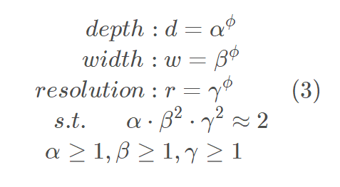
It should be noted that:
(1) The relationship between FLOPs and depth is that when depth is doubled, FLOPs is doubled.
(2) The relationship between FLOPs and width is that when the width is doubled (i.e. the channel is doubled), the FLOPs will be doubled by 4 times, because the FLOPs of the convolution layer is about equal to f e a t u r e W × f e a t u r e H × f e a t u r e C × k e r n e l W × k e r n e l H × k e r n e l n u m b e r feature_W×feature_H×feature_C×kernel_W×kernel_H×kernel_number featureW​ × featureH​ × featureC​ × kernelW​ × kernelH​ × kerneln_number (assuming that the height and width of the input and output characteristic matrix remain unchanged), when the width is doubled, the channels (feature_C) of the input characteristic matrix and the number of channels or convolution kernels (kernel_number) of the output characteristic matrix will be doubled, so the FLOPs will be doubled by four times.
(3) The relationship between FLOPs and resolution is that when the resolution is doubled, FLOPs will also be doubled by 4 times, which is similar to the above because of the width of the characteristic matrix f e a t u r e W feature_W Height of feature w # and feature matrix f e a t u r e H feature_H Feature h # will double.
Therefore, the magnification of the total FLOPS can be used ( α ⋅ β 2 ⋅ γ 2 ) ϕ (α⋅β^2⋅γ ^2)^ϕ ( α ⋅ β 2⋅ γ 2) ϕ To indicate when the limit ( α ⋅ β 2 ⋅ γ 2 ) (α⋅β^2⋅γ ^2) ( α ⋅ β 2⋅ γ 2) When it's about 2, for any one ϕ The number of FLOPS has increased 2 ϕ 2^ϕ two ϕ Times.

Next, the author uses NAS to search on the benchmark network efficientbet0-0 α , β , γ These three parameters,
(1) First fix ϕ = 1 \phi=1 ϕ= 1. Based on the above formulas (2) and (3), the author finds that the best parameter for efficientbet0 is α = 1.2 , β = 1.1 , γ = 1.15 \alpha=1.2, \beta=1.1, \gamma=1.15 α=1.2,β=1.1,γ=1.15 .
(2) Then fixed α = 1.2 , β = 1.1 , γ = 1.15 \alpha=1.2, \beta=1.1, \gamma=1.15 α= 1.2, β= 1.1, γ= 1.15, using different methods based on efficientbet0 ϕ \phi ϕ Efficientbet1 to efficientbet7 were obtained, respectively.
It should be noted that for different benchmark networks α , β , γ \alpha, \beta, \gamma α,β,γ Not necessarily the same. It should also be noted that in the original paper, the author also said that if you search directly on the large model α , β , γ \alpha, \beta, \gamma α,β,γ Better results may be obtained, but the search cost is too high in the larger model, so this article searches on the smaller efficient netb-0 model.

2. Detailed network structure

The following table shows the network framework of EfficientNet-B0 (B1-B7 is to modify Resolution, channels and Layers on the basis of B0). It can be seen that the network is divided into nine stages. The first stage is a common convolution layer with convolution core size of 3x3 and step length of 2 (including BN and activation function Swish). Stage2 ~ Stage8 are stacking MBConv structures repeatedly (the Layers in the last column indicate how many times the MBConv structure is repeated in the stage), and stage 9 consists of an ordinary 1x1 convolution layer (including BN and activation function Swish) consists of an average pooling layer and a full connection layer. Each MBConv in the table will be followed by a number 1 or 6, where 1 or 6 is the magnification factor n, that is, the first 1x1 convolution layer in MBConv will expand the channels of the input characteristic matrix to n times, where k3x3 or k5x5 represents the convolution kernel size adopted by Depthwise Conv in MBConv. Channels represents pass After this stage, the channels of the characteristic matrix are output.

From the above figure, we can find that the entire EfficientNet consists of seven parts of MBConv, corresponding to the MBConv in the above figure S t a g e 1 − S t a g e 7 Stage_1-Stage_7 Stage1 − Stage7. The specific parameters are as follows:

BlockArgs(kernel_size=3, num_repeat=1, input_filters=32, output_filters=16, expand_ratio=1, id_skip=True, stride=[1], se_ratio=0.25), 
BlockArgs(kernel_size=3, num_repeat=2, input_filters=16, output_filters=24, expand_ratio=6, id_skip=True, stride=[2], se_ratio=0.25), 
BlockArgs(kernel_size=5, num_repeat=2, input_filters=24, output_filters=40, expand_ratio=6, id_skip=True, stride=[2], se_ratio=0.25), 
BlockArgs(kernel_size=3, num_repeat=3, input_filters=40, output_filters=80, expand_ratio=6, id_skip=True, stride=[2], se_ratio=0.25), 
BlockArgs(kernel_size=5, num_repeat=3, input_filters=80, output_filters=112, expand_ratio=6, id_skip=True, stride=[1], se_ratio=0.25), 
BlockArgs(kernel_size=5, num_repeat=4, input_filters=112, output_filters=192, expand_ratio=6, id_skip=True, stride=[2], se_ratio=0.25), 
BlockArgs(kernel_size=3, num_repeat=1, input_filters=192, output_filters=320, expand_ratio=6, id_skip=True, stride=[1], se_ratio=0.25)]

GlobalParams(batch_norm_momentum=0.99, batch_norm_epsilon=0.001, dropout_rate=0.2, num_classes=1000, width_coefficient=1.0, 
            depth_coefficient=1.0, depth_divisor=8, min_depth=None, drop_connect_rate=0.2, image_size=224)

MBConv structure

MBConv is actually the inverted residualblock in MobileNetV3 network, but there are some differences. One is that the activation functions are different (Swish activation functions are used in MBConv of EfficientNet), and the other is that SE (sequence and exception) module is added to each MBConv.

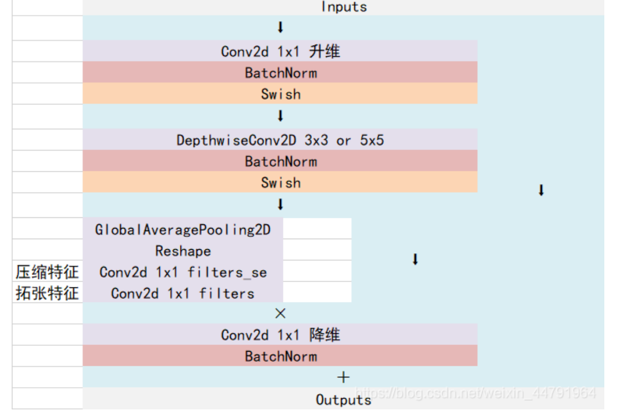
As shown in the figure, the MBConv structure is mainly composed of a 1x1 ordinary convolution (dimensionality increasing effect, including BN and Swish), a kxk depth conv convolution (including BN and Swish). The specific value of k can be seen. The network framework of EfficientNet-B0 mainly includes 3x3 and 5x5, including an SE module, a 1x1 ordinary convolution (dimensionality reducing effect, including BN) and a droopout layer.

be careful:
(1) The number of convolution kernels of the first 1x1 convolution layer is n times that of the input characteristic matrix channel, n ∈ { 1 , 6 } n \in \left\{1, 6\right\} n∈{1,6}.
(2) When n = 1, do not use the 1x1 convolution of the first dimension increase, that is, the MBConv structure does not have the 1x1 convolution of the first dimension increase
(3) In the shortcut, it can be used only when the stripe of depthwise conv in the MBConv structure is 1 and the number of input filters is equal to the number of output filters.
(4) In the SE module, the first 1 × The channel of 1 convolution is the channel of the MBConv characteristic matrix 1 4 \frac{1}{4} 41, and use Swish to activate the function. Second 1 × 1 the convoluted channel is equal to the characteristic matrix channels output by the Depthwise Conv layer, and the Sigmoid activation function is used.

class MBConvBlock(nn.Module):
    '''
    EfficientNet-b0:
    [BlockArgs(kernel_size=3, num_repeat=1, input_filters=32, output_filters=16, expand_ratio=1, id_skip=True, stride=[1], se_ratio=0.25), 
     BlockArgs(kernel_size=3, num_repeat=2, input_filters=16, output_filters=24, expand_ratio=6, id_skip=True, stride=[2], se_ratio=0.25), 
     BlockArgs(kernel_size=5, num_repeat=2, input_filters=24, output_filters=40, expand_ratio=6, id_skip=True, stride=[2], se_ratio=0.25), 
     BlockArgs(kernel_size=3, num_repeat=3, input_filters=40, output_filters=80, expand_ratio=6, id_skip=True, stride=[2], se_ratio=0.25), 
     BlockArgs(kernel_size=5, num_repeat=3, input_filters=80, output_filters=112, expand_ratio=6, id_skip=True, stride=[1], se_ratio=0.25), 
     BlockArgs(kernel_size=5, num_repeat=4, input_filters=112, output_filters=192, expand_ratio=6, id_skip=True, stride=[2], se_ratio=0.25), 
     BlockArgs(kernel_size=3, num_repeat=1, input_filters=192, output_filters=320, expand_ratio=6, id_skip=True, stride=[1], se_ratio=0.25)]
    
    GlobalParams(batch_norm_momentum=0.99, batch_norm_epsilon=0.001, dropout_rate=0.2, num_classes=1000, width_coefficient=1.0, 
                    depth_coefficient=1.0, depth_divisor=8, min_depth=None, drop_connect_rate=0.2, image_size=224)
    '''
    def __init__(self, block_args, global_params):
        super().__init__()
        self._block_args = block_args
        # Obtain standardized parameters
        self._bn_mom = 1 - global_params.batch_norm_momentum
        self._bn_eps = global_params.batch_norm_epsilon

        # Scaling of attention mechanism
        self.has_se = (self._block_args.se_ratio is not None) and (
            0 < self._block_args.se_ratio <= 1)
        # Do you need a short leg
        self.id_skip = block_args.id_skip 

        Conv2d = get_same_padding_conv2d(image_size=global_params.image_size)

        # 1x1 convolution channel expansion
        inp = self._block_args.input_filters  # number of input channels
        oup = self._block_args.input_filters * self._block_args.expand_ratio  # number of output channels
        if self._block_args.expand_ratio != 1:
            self._expand_conv = Conv2d(
                in_channels=inp, out_channels=oup, kernel_size=1, bias=False)
            self._bn0 = nn.BatchNorm2d(
                num_features=oup, momentum=self._bn_mom, eps=self._bn_eps)

        # Deep separable convolution
        k = self._block_args.kernel_size
        s = self._block_args.stride
        self._depthwise_conv = Conv2d(
            in_channels=oup, out_channels=oup, groups=oup,
            kernel_size=k, stride=s, bias=False)
        self._bn1 = nn.BatchNorm2d(
            num_features=oup, momentum=self._bn_mom, eps=self._bn_eps)

        # The attention mechanism module group first contracted the number of channels, and then expanded the number of channels
        if self.has_se:
            num_squeezed_channels = max(
                1, int(self._block_args.input_filters * self._block_args.se_ratio))
            self._se_reduce = Conv2d(
                in_channels=oup, out_channels=num_squeezed_channels, kernel_size=1)
            self._se_expand = Conv2d(
                in_channels=num_squeezed_channels, out_channels=oup, kernel_size=1)

        # Output part
        final_oup = self._block_args.output_filters
        self._project_conv = Conv2d(
            in_channels=oup, out_channels=final_oup, kernel_size=1, bias=False)
        self._bn2 = nn.BatchNorm2d(
            num_features=final_oup, momentum=self._bn_mom, eps=self._bn_eps)
        self._swish = MemoryEfficientSwish()

    def forward(self, inputs, drop_connect_rate=None):
        x = inputs
        if self._block_args.expand_ratio != 1:
            x = self._swish(self._bn0(self._expand_conv(inputs)))

        x = self._swish(self._bn1(self._depthwise_conv(x)))

        # Added attention mechanism
        if self.has_se:
            x_squeezed = F.adaptive_avg_pool2d(x, 1)
            x_squeezed = self._se_expand(
                self._swish(self._se_reduce(x_squeezed)))
            x = torch.sigmoid(x_squeezed) * x

        x = self._bn2(self._project_conv(x))

        # The short circuit can be performed only when the following conditions are met
        input_filters, output_filters = self._block_args.input_filters, self._block_args.output_filters
        if self.id_skip and self._block_args.stride == 1 and input_filters == output_filters:
            if drop_connect_rate:
                x = drop_connect(x, p=drop_connect_rate,
                                 training=self.training)
            x = x + inputs  # skip connection
        return x

    def set_swish(self, memory_efficient=True):
        """Sets swish function as memory efficient (for training) or standard (for export)"""
        self._swish = MemoryEfficientSwish() if memory_efficient else Swish()

3. Detailed parameters of efficientbetnet-0 ~ B-7

Among them,
(1) input_size represents the image size of the input network when training the network
(2) width_coefficient represents the magnification factor in the channel dimension. For example, in efficientbet0, the number of convolution cores used in the 3x3 convolution layer of Stage 1 is 32, so it is 32 in B6 × 1.8 = 57.6, and then rounded to the nearest integer multiple of 8, i.e. 56. The same is true for other stages.
(3) depth_coefficient represents the magnification factor on the depth dimension (only for Stage2 to Stage8), such as Stage7 in efficientbet0 L ^ i = 4 \hat L_i=4 L^i = 4, then it is 4 in B6 × 2.6 = 10.4 then rounded up, i.e. 11.
(4) Drop_connect_rate is the drop_rate used in the dropout layer of the MBConv structure. In the implementation of the official keras module, the drop_rate of the MBConv structure increases from 0 to drop_connect_rate (see the official source code for the specific implementation. Note that the dropout layer is only available when using shortcut in the source code implementation). It should also be noted that the dropout layer here is Stochastic Depth, that is, the main branch of the whole block will be lost randomly (only the shortcut branch is left, which is equivalent to directly skipping this block). It can also be understood as reducing the depth of the network.
(5) Dropout_rate is the dropout_rate of the dropout layer before the last full connection layer (between Pooling and FC of stage9).

4. Experimental results