1, Introduction

1 PCA
PCA (Principal Component Analysis) is a commonly used data analysis method. PCA is a method that transforms the original data into a group of data representation with linear independence of each dimension through linear transformation. It can be used to extract the main feature components of data and is often used for dimensionality reduction of high-dimensional data.

1.1 dimensionality reduction
In data mining and machine learning, data is represented by vectors. For example, the flow and transaction of a Taobao store in 2012 can be regarded as a set of records, in which the data of each day is a record, and the format is as follows:
(date, number of views, number of visitors, number of orders, number of transactions, transaction amount)
Where "date" is a record flag rather than a measure, and data mining is mostly concerned with measures. Therefore, if we ignore the field of date, we get a group of records. Each record can be expressed as a five-dimensional vector, and one sample is as follows:

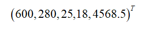
Generally, it is customary to use column vectors to represent a record, and this criterion will be followed later in this article.
The complexity of many machine learning algorithms is closely related to the dimension of data, and even exponentially related to the dimension. It may not matter that there are only 5-Dimensional data here, but it is not uncommon to process thousands or even tens of thousands of dimensional data in actual machine learning. In this case, the resource consumption of machine learning is unacceptable, so the dimension reduction operation will be taken on the data. Dimensionality reduction means the loss of information. However, in view of the correlation of the actual data itself, we should find ways to reduce the loss of information.
For example, according to the data of Taobao stores above, it is known from experience that "views" and "number of visitors" often have a strong correlation, while "number of orders" and "number of transactions" also have a strong correlation. It can be intuitively understood as "when the number of visitors to this store is high (or low) on a certain day, we should largely think that the number of visitors on that day is also high (or low)". Therefore, if you delete the number of views or visitors, you will not lose too much information in the end, thus reducing the dimension of the data, which is the so-called dimensionality reduction operation. If data dimensionality reduction is analyzed and discussed in mathematics, it is PCA in professional terms, which is a dimensionality reduction method with strict mathematical basis and has been widely used.

1.2 vector and base transformation
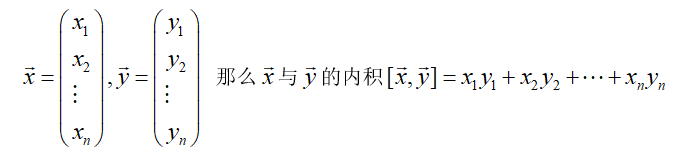
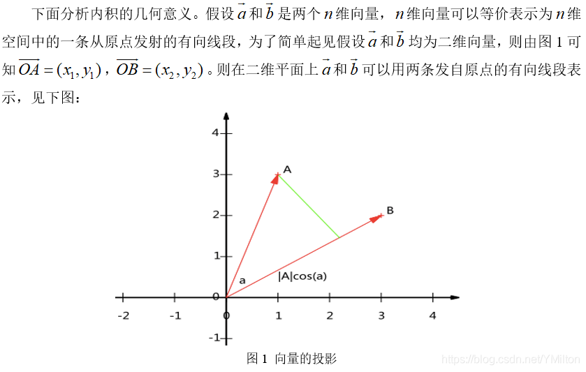
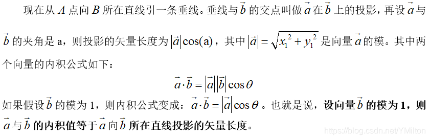
1.2.1 inner product and projection
The inner product of two vectors of the same size is defined as follows:



1.2.2 Foundation
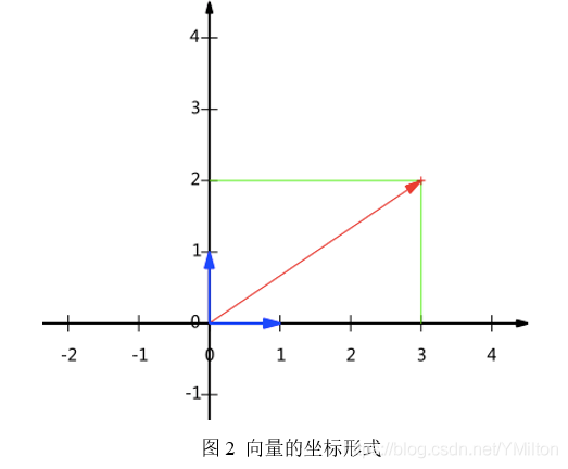
In algebra, the vector is often represented by the point coordinates of the end of the line segment. Suppose the coordinates of a vector are (3,2), where 3 actually means that the projection value of the vector on the x-axis is 3 and the projection value on the y-axis is 2. In other words, a definition is implicitly introduced: take the vector with the length of 1 in the positive direction on the x-axis and y-axis as the standard. Then a vector (3,2) actually has a projection of 3 on the x-axis and 2 on the y-axis. Note that the projection is a vector and can be negative. The vector (x, y) actually represents a linear combination:

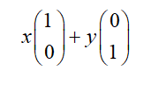
From the above representation, it can be obtained that all two-dimensional vectors can be expressed as such a linear combination. Here (1,0) and (0,1) are called a set of bases in two-dimensional space.

The reason why (1,0) and (0,1) are selected as the basis by default is of course for convenience, because they are the unit vectors in the positive direction of x and y axes respectively, so the point coordinates and vectors on the two-dimensional plane correspond one to one. But in fact, any two linearly independent two-dimensional vectors can become a set of bases. The so-called linearly independent in the two-dimensional plane is intuitively two vectors that are not in a straight line.

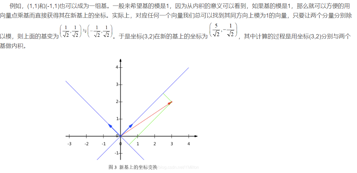
In addition, the bases here are orthogonal (i.e. the inner product is 0, or intuitively perpendicular to each other). The only requirement for a group of bases is that they are linearly independent, and non orthogonal bases are also acceptable. However, because orthogonal bases have good properties, the commonly used bases are orthogonal.
1.2.3 matrix of base transformation
The base transformation in the above example can be expressed by matrix multiplication, that is

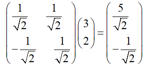
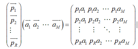
If we generalize it, suppose there are m N-dimensional vectors and want to transform them into a new space represented by R N-dimensional vectors, then first form matrix A by rows, and then form matrix B by columns. Then the product ab of the two matrices is the transformation result, in which the m-th column of AB is the transformation result of the m-th column of a, which is expressed by matrix multiplication as:


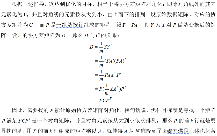
1.3 covariance matrix and optimization objectives
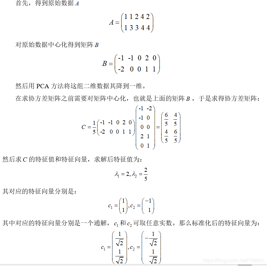
In data dimensionality reduction, the key problem is how to determine the optimal basis. In other words, selecting the optimal basis is to ensure the characteristics of the original data to the greatest extent. Here, it is assumed that there are 5 pieces of data

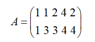
Calculate the average value of each row, and then subtract the average value from each row to obtain

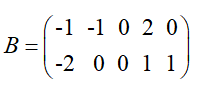
The matrix is represented in the form of coordinates, and the figure is as follows:

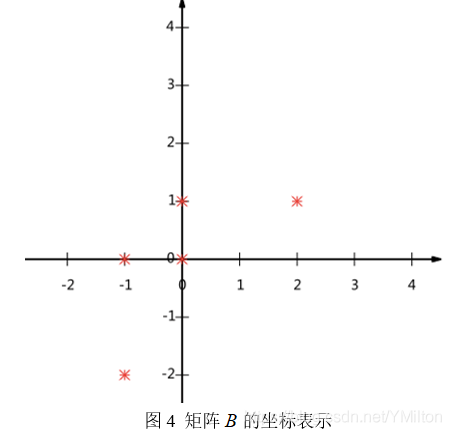
So the question now is: how to choose to use one-dimensional vector to represent these data and hope to retain the original information as much as possible? In fact, this problem is to select a vector in one direction in the two-dimensional plane, project all data points onto this line, and use the projected value to represent the original record, that is, the problem of reducing two-dimensional to one-dimensional. So how to choose this direction (or base) to retain the most original information? An intuitive view is that we want the projection value after projection to be as scattered as possible.

1.3.1 variance
The above problem is that it is hoped that the projected value after projection will be dispersed in one direction as much as possible, and this degree of dispersion can be expressed by mathematical variance, that is:

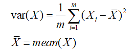
Therefore, the above problem is formally expressed as: find a wiki so that after all data are transformed into coordinates on this basis, the variance value is the largest.

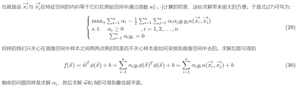
2.3.2 covariance
Mathematically, the correlation can be expressed by the covariance of two characteristics, namely:

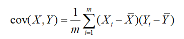
When the covariance is 0, the two features are completely independent. In order to make the covariance 0, the second base can only be selected in the direction orthogonal to the first base. Therefore, the two directions finally selected must be orthogonal.

So far, the optimization objective of the dimensionality reduction problem is obtained: reduce a group of N-dimensional vectors to k-dimensional (k < N). Its goal is to select k unit (modulus 1) orthogonal bases, so that after the original data is transformed to this group of bases, the covariance between each field is 0, and the variance of the field is as large as possible (under the constraint of orthogonality, the maximum K variances are taken).

2.3.3 covariance matrix
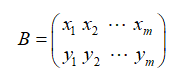
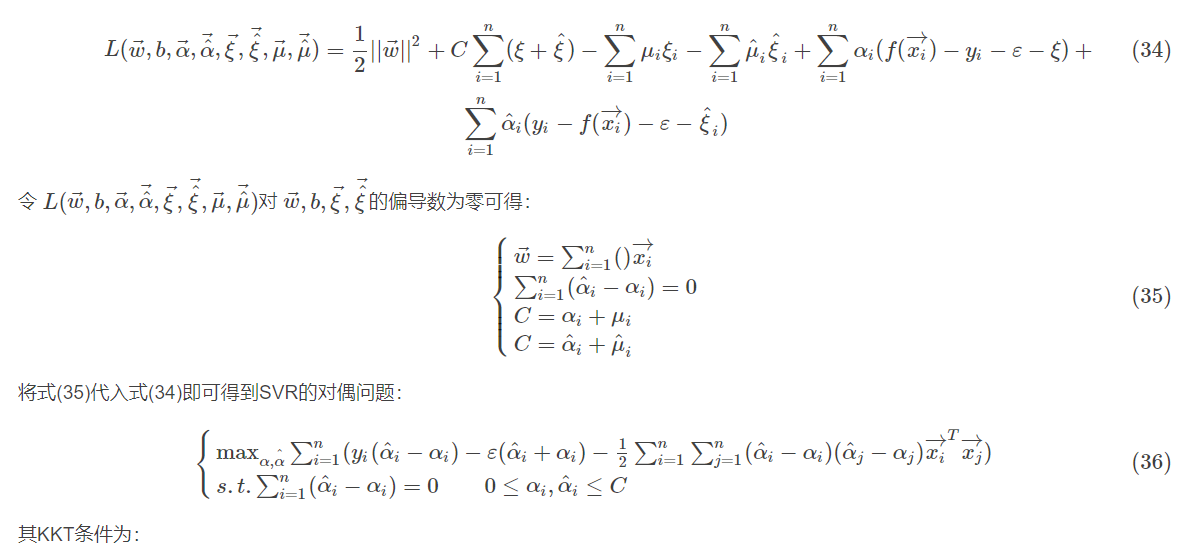
Assuming that there are only two fields x and y, they form a matrix according to rows, which is the matrix obtained by subtracting the average value of each field from each field through the centralized matrix:


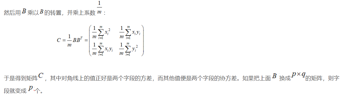
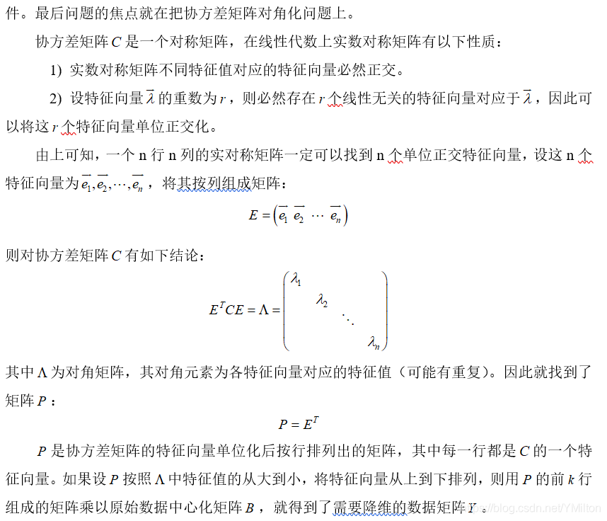
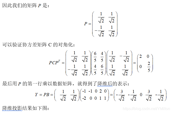
3.4 diagonalization of covariance matrix


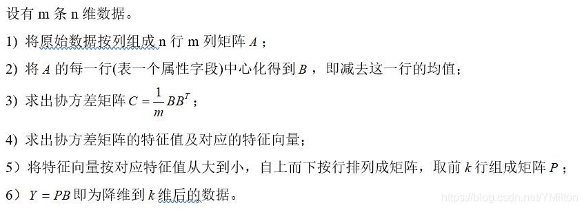
1.4 algorithms and examples
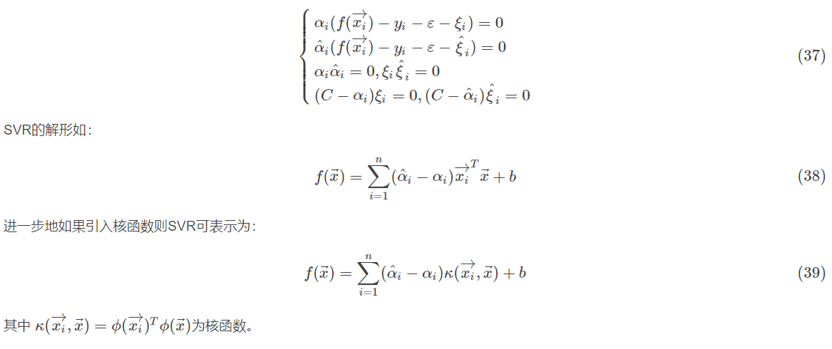
1.4.1 PCA algorithm

1.4.2 examples


1.5. discuss
According to the above explanation of the mathematical principle of PCA, we can understand some capabilities and limitations of PCA. PCA essentially takes the direction with the largest variance as the main feature, and "decorrelates" the data in each orthogonal direction, that is, they have no correlation in different orthogonal directions.

Therefore, PCA also has some limitations. For example, it can well remove linear correlation, but there is no way for high-order correlation. For data with high-order correlation, Kernel PCA can be considered to convert nonlinear correlation into linear correlation through Kernel function. In addition, PCA assumes that the main features of the data are distributed in the orthogonal direction. If there are several directions with large variance in the non orthogonal direction, the effect of PCA will be greatly reduced.

Finally, it should be noted that PCA is a parameter free technology, that is, in the face of the same data, if you do not consider cleaning, the results will be the same who will do it, and there is no intervention of subjective parameters. Therefore, PCA is convenient for general implementation, but it cannot be personalized optimization.

2 basic concepts of SVM
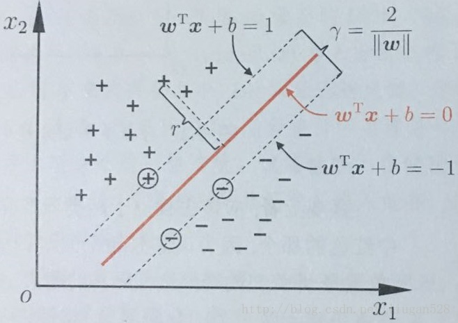
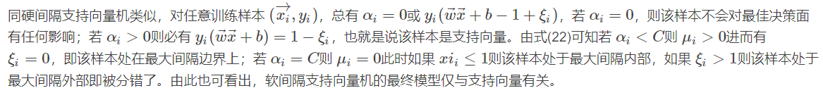
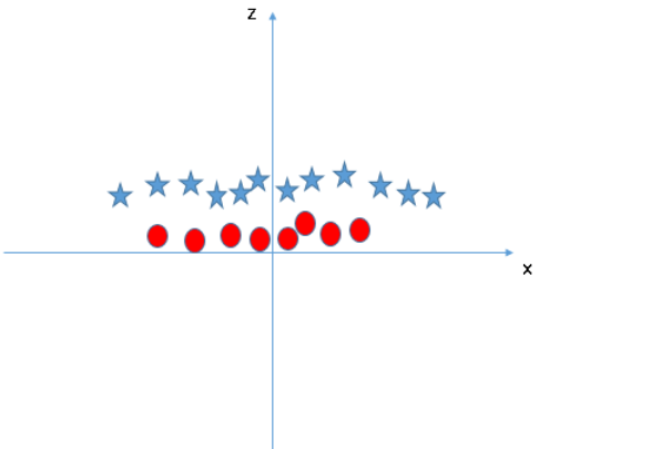
The basic model of support vector machine (SVM) is to find the best separation hyperplane in the feature space to maximize the interval between positive and negative samples on the training set. After the introduction of SVM kernel learning algorithm, SVM can also be used to solve the problem.
There are three types of general SVM:

Hard interval support vector machine (linearly separable support vector machine): when the training data is linearly separable, a linearly separable support vector machine can be obtained by maximizing the hard interval.
Soft interval support vector machine: when the training data is approximately linearly separable, a linear support vector machine can be obtained through the maximum chemistry of soft interval.
Nonlinear support vector machine: when the training data is linearly inseparable, a nonlinear support vector machine can be obtained by kernel method and soft interval maximum chemistry.

2.2 hard interval support vector machine


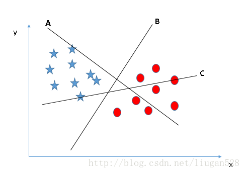
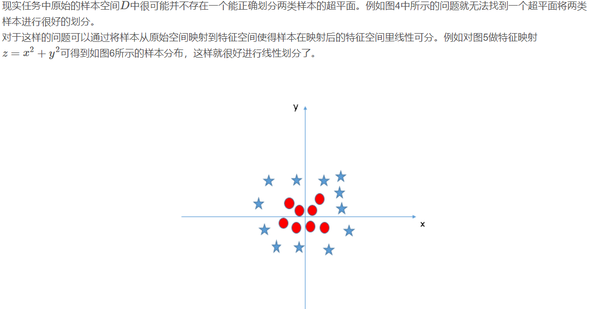
For the three hyperplanes A, B and C in Fig. 2, hyperplane C should be selected, because using hyperplane C for division has the best "tolerance" to the local disturbance of training samples and the strongest robustness of classification. For example, due to the limitations of the training set or the interference of noise, the samples outside the training set may be closer to the current separation boundary of the two classes than the training samples in Figure 2, and errors will occur in the classification decision-making, while hyperplane C is least affected, that is to say, the classification results generated by hyperplane C are the most robust and credible, and the generalization ability of unseen samples is the strongest.

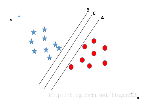
The best hyperplane is derived from the example in the figure below.



This is the basic type of SVM.

2.2.1 Lagrangian duality problem


2.2.2 KKT condition of SVM problem

2.3 soft interval support vector machine




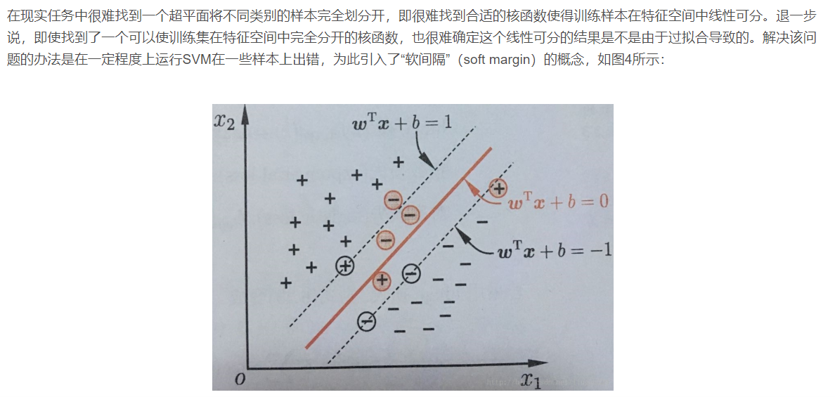
2.4 nonlinear support vector machine




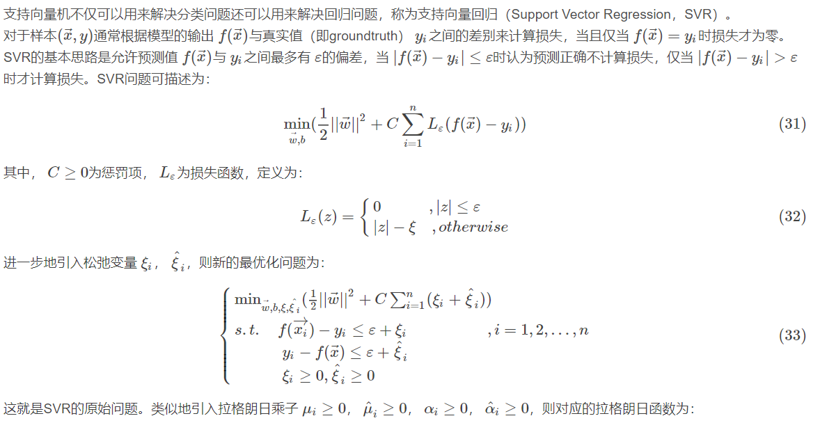
2.4.1 support vector regression



2.4.2 common kernel functions

2.5 advantages and disadvantages of SVM
advantage:
SVM is easy to get the nonlinear relationship between data and features when the sample size is small and medium. It can avoid the problem of neural network structure selection and local minimum. It has strong interpretability and can solve high-dimensional problems.
Disadvantages:
SVM is sensitive to missing data and has no general solution to nonlinear problems. The correct selection of kernel function is not easy and the computational complexity is high. The mainstream algorithm can reach the complexity of O(n2)O(n2), which is unbearable for large-scale data.

2, Source code

function varargout = test(varargin)
gui_Singleton = 1;
gui_State = struct('gui_Name',       mfilename, ...
                   'gui_Singleton',  gui_Singleton, ...
                   'gui_OpeningFcn', @test_OpeningFcn, ...
                   'gui_OutputFcn',  @test_OutputFcn, ...
                   'gui_LayoutFcn',  [] , ...
                   'gui_Callback',   []);
if nargin && ischar(varargin{1})
    gui_State.gui_Callback = str2func(varargin{1});
end

if nargout
    [varargout{1:nargout}] = gui_mainfcn(gui_State, varargin{:});
else
    gui_mainfcn(gui_State, varargin{:});
end

function test_OpeningFcn(hObject, eventdata, handles, varargin)
global imgrow imgcol V pcaface accuracy
imgrow=112;
imgcol=92;%The read image is 112*92
npersons=41;%Select the faces of 41 people
disp('Read training data...');
f_matrix=ReadFace(npersons,0);%Read training data
nfaces=size(f_matrix,1);%Number of sample faces

%The image in low dimensional space is( npersons*5)*k Each row represents a principal component face, and each face has 20 dimensional features
disp('Training data PCA feature extraction ...');
mA=mean(f_matrix);%Find the mean value of each attribute
k=20;%Dimension reduction to 20 dimensions
[pcaface,V]=fastPCA(f_matrix,k,mA);%Principal component analysis feature extraction
%pcaface It's 200*20
disp('Normalization of training characteristic data....')
lowvec=min(pcaface);
upvec=max(pcaface);
scaledface=scaling(pcaface,lowvec,upvec);

disp('SVM Sample training...')
gamma=0.0078;
c=128;
multiSVMstruct=multiSVMtrain(scaledface,npersons,gamma,c);
save('recognize.mat','multiSVMstruct','npersons','k','mA','V','lowvec','upvec');

disp('Read test data...')
[testface,realclass]=ReadFace(npersons,1);

disp('Dimensionality reduction of test data...')
m=size(testface,1);
for i=1:m
    testface(i,:)=testface(i,:)-mA;
end
pcatestface=testface*V;
disp('Standardization of test characteristic data...')
scaledtestface=scaling(pcatestface,lowvec,upvec);
disp('Sample classification...')
class=multiSVM(scaledtestface,multiSVMstruct,npersons);

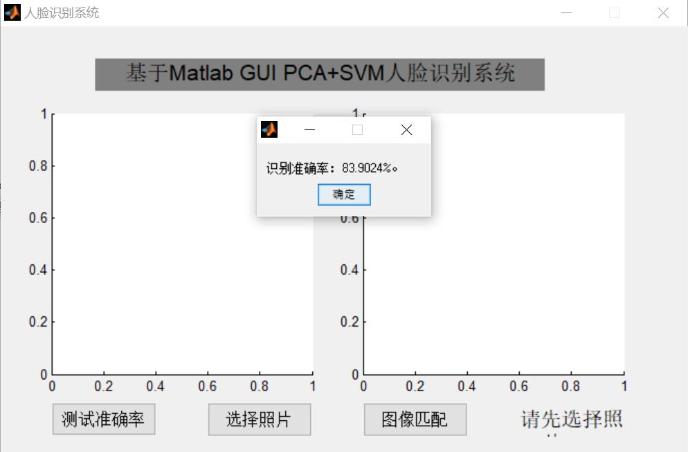
disp('Test complete!')
accuracy=sum(class==realclass)/length(class);
set(handles.change_font,'string','Please select photos first......')
handles.output = hObject;
guidata(hObject, handles);
function [f_matrix,realclass]=ReadFace(npersons,flag)
%read ORL Data from face database photos to matrix
%Input:
%    npersons-The number of people to be read. The first five pictures of each person are training samples and the last five are verification samples
%    imgrow-The row pixels of the image are global variables
%    imgcol-The column pixels of the image are global variables
%    flag-Flag, 0 means reading training samples, 1 means reading test samples
%Output:
%Known global variables: imgrow=112;imgcol=92;
global imgrow;
global imgcol;
realclass=zeros(npersons*5,1);%zeros Creating an all zero array matrix creates a 200*1 Zero matrix of
f_matrix=zeros(npersons*5,imgrow*imgcol);%Created a 200*(112*92)Put all the faces in the training set on this zero matrix f_matrix in
for i=1:npersons
    facepath='./orl_faces/s';%Path of training sample set
    facepath=strcat(facepath,num2str(i));%strcat String splicing num2str()Convert a number to a string
    facepath=strcat(facepath,'/');
    cachepath=facepath;%Get the path of the picture
    for j=1:5
    unction [ scaledface] = scaling( faceMat,lowvec,upvec )
%Feature data normalization
%input??faceMat Image data that needs to be normalized,
%       lowvec Original minimum
%       upvec Original maximum
upnew=1;
lownew=-1;
[m,n]=size(faceMat);
scaledface=zeros(m,n);
for i=1:m
    scaledface(i,:)=lownew+(faceMat(i,:)-lowvec)./(upvec-lowvec)*(upnew-lownew);
end
end
voting=zeros(m,nclass);
for i=1:nclass-1
    for j=i+1:nclass
        class=svmclassify(multiSVMstruct{i}{j},testface);
        voting(:,i)=voting(:,i)+(class==1);
        voting(:,j)=voting(:,j)+(class==0);
    end
end
[~,class]=max(voting,[],2);
end

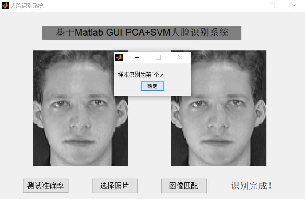
3, Operation results

4, Remarks

Complete code or write on behalf of QQ 912100926