Pulse compression / matched filter is one of the most basic operations of radar signal processing. This paper deduces the basic principle of matched filter in detail, and gives the simulation program of matlab.

Because there are too many formulas, we share them here in the form of screenshots. If you need word or pdf, you can leave a message or private letter.

Basic principle of pulse compression

 

 

 

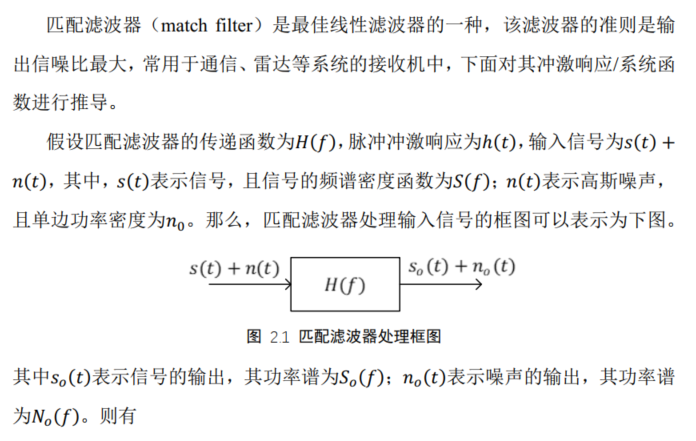
Time domain matched domain filtering

 

 

 

 

 

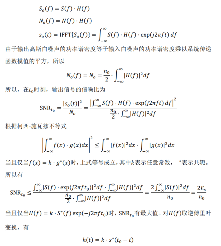
Frequency domain matched filtering

Implementation of matched filtering

Synthetic aperture radar imaging - algorithm and implementation introduces three implementation methods of matched filtering. The relevant codes are as follows

(Simulation figure 3.13 of synthetic aperture radar imaging - algorithm and implementation [10]_ Destiny0321 column - CSDN blog)

% SAR_Figure_3_13
% 2016/08/31
close all;clear all;clc;

T = 10e-6;          % Pulse duration
B = 15e6;           % Pulse bandwidth
K = B/T;            % Frequency modulation rate
ratio = 5;          % Oversampling rate
Fs = ratio*B;       % sampling frequency 
dt = 1/Fs;          % Sampling interval
Nr = ceil(T/dt);    % Sampling points
t0 = ((0:Nr-1)-Nr/2)/Nr*T;          % Basic timeline

st0 = exp(1i*pi*K*(t0-T/5).^2);     % Basic signal
space1 = zeros(1,round(Nr/5));      % Generate null signal
space2 = zeros(1,Nr);               % Generate null signal
st = [space1,st0,space2,st0,space2,st0,space1];     % Actual signal

N = length(st);             % Actual signal length
n = 0:N-1;                  % Sample axis
f = ((0:N-1)-N/2)/N*Fs;     % Fundamental frequency axis

Sf = fftshift(fft(st));                         % Fourier transform of real signal
Hf1 = fftshift(fft(conj(fliplr(st0)),N));       % Matched filter of mode 1: take complex conjugate after time deconvolution and calculate N Point zero DFT
Hf2 = fftshift(conj(fft(st0,N)));               % Matched filter of mode 2: calculation after zeroing DFT，Complex conjugate of the result
Hf3 = exp(1i*pi*f.^2/K);                        % Matched filter of mode 3: directly generate matched filter in frequency domain

out1 = ifft(ifftshift(Sf.*Hf1));
out2 = ifft(ifftshift(Sf.*Hf2));
out3 = ifft(ifftshift(Sf.*Hf3));

figure,set(gcf,'Color','w');
subplot(4,1,1),plot(n,real(st));axis tight
title('(a)Real part of input array signal');ylabel('range');
subplot(4,1,2),plot(n,abs(out1));axis tight
title('(b)Matched filter output of mode 1');ylabel('range');
subplot(4,1,3),plot(n,abs(out2));axis tight
title('(c)Mode 2 matched filter output');ylabel('range');
subplot(4,1,4),plot(n,abs(out3));axis tight
title('(d)Matched filter output of mode 3');xlabel('time(Sampling point)');ylabel('range');

%%
figure, plot(abs(fft(st0)))

%% 
NN = length(st);
fr = [0:NN/2-1, -NN/2:-1]/NN*Fs;
Hr = exp(-j*pi*fr.^2/K);
src1 = ifft(fft(st).*Hr);
figure, plot(abs(src1))

The running results of the above code are shown in the figure below.

Problems in the above simulation: in the actual radar signal processing, we can not get st0 in the above code.

On the premise that the radar signal waveform is known, matched filtering can be carried out in time domain or frequency domain. However, in actual SAR signal processing, matched filtering is mostly carried out in frequency domain for two main reasons:

1. Convolution operation is required in time domain, and the amount of computation is large; Only Fourier transform and complex multiplication are needed in frequency domain, which has high efficiency;
2. A pulse of the actual SAR signal contains the transmitted signal of the target within the whole width, so the length of the filter is far greater than the length of the actual transmitted signal. In order to improve the efficiency of time-domain matched filtering, the length of the designed matched filter is usually consistent with the transmitted signal.

To sum up, assuming that the length of a radar signal is n and the radar waveform is known, we can directly construct an ideal signal with length N in time domain or frequency domain, and then construct a matched filter. The code is as follows:

close all;clear all;clc;

T = 10e-6;          % Pulse duration
B = 15e6;           % Pulse bandwidth
K = B/T;            % Frequency modulation rate
ratio = 1.2;          % Oversampling rate
Fs = ratio*B;       % sampling frequency 
dt = 1/Fs;          % Sampling interval
Nr = 8192;
tr = [-Nr/2:Nr/2-1]/Fs;

st = zeros(1, Nr);

for ii = -15:15
    tr1 = tr + ii*T;
    st0 = (abs(tr1)<T/2).*exp(-j*pi*K*tr1.^2);
    st = st + st0;
end

figure, plot(real(st));
figure, plot(abs(fftshift(fft(st))))

%%
NN = Nr;
fr = [0:NN/2-1, -NN/2:-1]/NN*Fs;
Hr = exp(-j*pi*fr.^2/K);
src1 = ifft(fft(st).*Hr);
figure, plot(abs(src1));

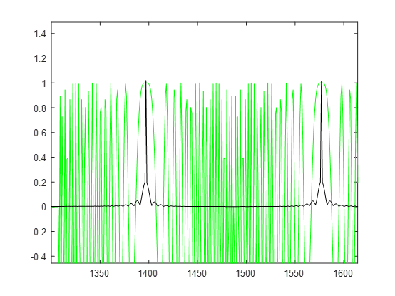
figure,  plot(real(st), 'y'); hold on
plot(abs(src1)/12, 'k');

After running the above code, the results are shown in the figure below. It can be seen that the pulse peak exactly corresponds to the zero frequency of LFM signal.