catalogue
4. Realize GWO algorithm with matlab code
1. Algorithm Introduction
Grey Wolf Optimizer (GWO) was proposed by Mirjalili in 2014. GWO algorithm is a new swarm intelligence optimization algorithm derived from simulating the social hierarchy mechanism and hunting behavior of grey wolf groups in nature. In GWO algorithm, each grey wolf represents a candidate solution in the population, and the optimal solution in the population is called α, The suboptimal solution is called β, The third optimal solution is called δ, Other solutions are called ω. The social hierarchy of gray wolf is shown in the figure:
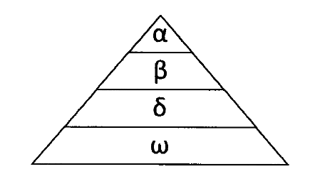
The social class can be divided into wolves α, Subordinate Wolf β, Ordinary Wolf δ And the bottom Wolf ω Four floors, including α Responsible for leading the wolves, β assist α Make decisions, δ obey α and β Can also command the underlying individuals ω. Application of grey wolf optimization algorithm α,β and δ Represent the historical optimal solution, suboptimal solution and third optimal solution respectively, ω Represents the remaining individuals. In the process of algorithm evolution, α,β and δ It is responsible for locating the position of prey and guiding other individuals to complete the behaviors of approaching, encircling and attacking, so as to finally achieve the purpose of preying on prey.
2. Algorithm principle
1) Gray wolf groups gradually approach and surround their prey through the following formulas:
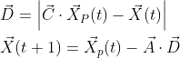
Where, t is the current iterative algebra, a and C are coefficient vectors, XP and X are the position vector of prey and the position vector of gray wolf respectively. A and C are calculated as follows:
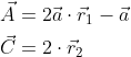

Where a is the convergence factor, and R1 and R2 obey the uniform distribution between [0,1] as the number of iterations decreases linearly from 2 to 0.
2) Other gray wolf individuals in the wolf pack Xi α,β And δ Position X of α, X β And X δ To update their respective locations.
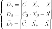
Where, D α, D β And D δ Respectively represent α,β and δ Distance from other individuals; X α, X β And X δ Respectively represent α,β and δ The current location of the; C1, C2 and C3 are random vectors, and X is the current gray wolf position.
The position update formula of gray wolf individuals is as follows:
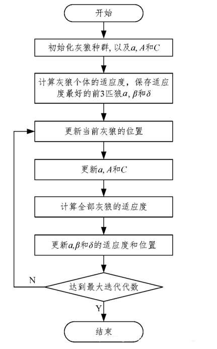
3. Implementation steps
Step 1: population initialization: including population number N, maximum number of iterations Maxlter, and control parameters a, a, C
Step 2: randomly initialize the position X of gray wolf individuals according to the upper and lower bounds of variables.
Step 3: calculate the fitness value of each wolf and save the location information of the wolf with the best fitness value in the population α, The location information of wolves with suboptimal fitness value in the population is saved as X β, The position information of the gray wolf with the third best fitness in the population is saved as X γ.
Step 4: update the position of gray wolf individual X.
Step 5: update parameters a, a and C.
Step 6: calculate the fitness value of each gray wolf and update the optimal position of the three wolves.
Step 7: judge whether the maximum number of iterations Maxlter is reached. If it is satisfied, the algorithm stops and returns X α As the final optimal solution, otherwise go to step 4.
4. Realize GWO algorithm with matlab code
4.1 main.m
% main program GWO
clear
close all
clc
SearchAgents_no = 30 ; % Population size
dim = 10 ; % Particle dimension
Max_iter = 1000 ; % Number of iterations
ub = 5 ;
lb = -5 ;
% Initialize the position of the three headed wolf
Alpha_pos=zeros(1,dim);
Alpha_score=inf;
Beta_pos=zeros(1,dim);
Beta_score=inf;
Delta_pos=zeros(1,dim);
Delta_score=inf;
%Initialize the location of the population
Positions = lb + rand(SearchAgents_no,dim).*(ub-lb) ; % Initialize the position of the particle swarm
Convergence_curve = zeros(Max_iter,1);
% Start cycle
for l=1:Max_iter
for i=1:size(Positions,1)
% Return back the search agents that go beyond the boundaries of the search space
Flag4ub=Positions(i,:)>ub;
Flag4lb=Positions(i,:)<lb;
Positions(i,:)=(Positions(i,:).*(~(Flag4ub+Flag4lb)))+ub.*Flag4ub+lb.*Flag4lb;
% Calculate objective function for each search agent
fitness=sum(Positions(i,:).^2);
% Update Alpha, Beta, and Delta
if fitness<Alpha_score
Alpha_score=fitness; % Update alpha
Alpha_pos=Positions(i,:);
end
if fitness>Alpha_score && fitness<Beta_score
Beta_score=fitness; % Update beta
Beta_pos=Positions(i,:);
end
if fitness>Alpha_score && fitness>Beta_score && fitness<Delta_score
Delta_score=fitness; % Update delta
Delta_pos=Positions(i,:);
end
end
a=2-l*((2)/Max_iter); % a decreases linearly fron 2 to 0
% Update the Position of search agents including omegas
for i=1:size(Positions,1)
for j=1:size(Positions,2)
r1=rand(); % r1 is a random number in [0,1]
r2=rand(); % r2 is a random number in [0,1]
A1=2*a*r1-a; % Equation (3.3)
C1=2*r2; % Equation (3.4)
D_alpha=abs(C1*Alpha_pos(j)-Positions(i,j)); % Equation (3.5)-part 1
X1=Alpha_pos(j)-A1*D_alpha; % Equation (3.6)-part 1
r1=rand();
r2=rand();
A2=2*a*r1-a; % Equation (3.3)
C2=2*r2; % Equation (3.4)
D_beta=abs(C2*Beta_pos(j)-Positions(i,j)); % Equation (3.5)-part 2
X2=Beta_pos(j)-A2*D_beta; % Equation (3.6)-part 2
r1=rand();
r2=rand();
A3=2*a*r1-a; % Equation (3.3)
C3=2*r2; % Equation (3.4)
D_delta=abs(C3*Delta_pos(j)-Positions(i,j)); % Equation (3.5)-part 3
X3=Delta_pos(j)-A3*D_delta; % Equation (3.5)-part 3
Positions(i,j)=(X1+X2+X3)/3;% Equation (3.7)
end
end
Convergence_curve(l)=Alpha_score;
disp(['Iteration = ' num2str(l) ', Evaluations = ' num2str(Alpha_score)]);
end
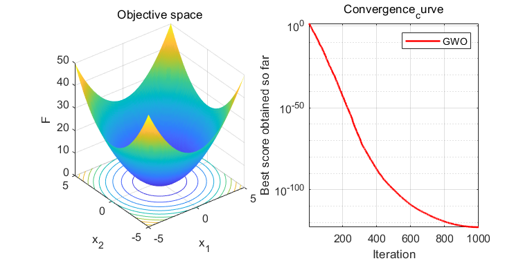
figure('unit','normalize','Position',[0.3,0.35,0.4,0.35],'color',[1 1 1],'toolbar','none')
subplot(1,2,1);
x = -5:0.1:5;y=x;
L=length(x);
f=zeros(L,L);
for i=1:L
for j=1:L
f(i,j) = x(i)^2+y(j)^2;
end
end
surfc(x,y,f,'LineStyle','none');
xlabel('x_1');
ylabel('x_2');
zlabel('F')
title('Objective space')
subplot(1,2,2);
semilogy(Convergence_curve,'Color','r','linewidth',1.5)
title('Convergence_curve')
xlabel('Iteration');
ylabel('Best score obtained so far');
axis tight
grid on
box on
legend('GWO')
display(['The best solution obtained by GWO is : ', num2str(Alpha_pos)]);
display(['The best optimal value of the objective funciton found by GWO is : ', num2str(Alpha_score)]);
References: seyedali mirjalili, Seyed Mohammad mirjalili, Andrew Lewis Grey Wolf Optimizer[J]. Advances in Engineering Software,2014,69.
4.2 operation results