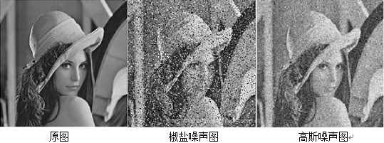
1. Adding noise to the image
Adding noise to an image can enhance the data
Adding a proper amount of noise to the training data can make the training model more robust and help to improve the performance of the model.
Two common noises: salt and pepper noise and Gaussian noise
import cv2
import numpy as np
import random
#Add salt and pepper noise
def salt_and_pepper_noise(img,percentage):
    rows,cols=img.shape
    num=int(percentage*rows*cols)
    for i in range(num):
        x=random.randint(0,rows-1)
        y=random.randint(0,cols-1)
        if random.randint(0,1)==0:
            img[x,y]=0    #Black Noise
        else:
            img[x,y]=255    #White Noise
     return img

 #Adding Gaussian Noise
 def gaussian_noise(img,mu,sigma,k):
     rows,cols=img.shape
     for i in range(rows):
         for j in range(cols):
             #Generate a random number with a Gaussian distribution that is rounded when added to the original data
             value=int(img[i,j]+k*random.gauss(mu=mu,sigma=sigma))
             #Limit the upper and lower boundaries of data values
             value=np.clip(a_max=255,a_min=0,a=value)
             img[i,j]=value
     return img

 img=cv2.imread('lena.jpg')

#Convert to Grayscale Image
gray_img=cv2.cvtColor(img,cv2.COLOR_BGR2GRAY)
cv2.imwrite('gray_lena.jpg',gray_img)
#You need to make a copy, or you can reference the image and the subsequent operations will overlap
gray_img2=gray_img.copy()

#Save salt and pepper noise image
cv2.imwrite('salt_and_pepper.jpg',salt_and_pepper_noise(gray_img,0.3))
#Save Gaussian Noise Image
cv2.imwrite('gaussian.jpg',gaussian_noise(gray_img2,0,1,32))

2. Image Filtering
1,2-Dimensional Convolution
cv2.filter2D(src,ddepth,kernel,dst,anchor,delta,borderType)
- src: Input Image
- ddepth: The desired depth for the target image, if -1 means that the input and output image depths are the same. (Image depth: the number of bits used to store each pixel)
- kernel:Convolutional kernel
- dst: Target image, same size and number of channels as original image
- Anchor: The base point (anchor point) of the kernel. The default values (-1, -1) indicate that the center of the core is the anchor point
- delta: similar to offset, default is 0
- borderType: Method of approaching pixels outward, default BORDER_DEFAULT
2. Median filter
cv2.medianBlur(src,ksize,dst) #Feature: The pixel of the center point is replaced by the pixel value of the median in the kernel
- src: original
- ksize: The size of the box, sorting the values in the box, taking the median as the current value
- dst: Target image, same size and number of channels as original image
3. Mean filter
cv2.blur(src,ksize,dst,anchor,borderType) #Replace the center pixel with the average value of all the pixels in the kernel area. The contribution rate of the core area is the same, which is good for salt and pepper noise.
- src: original
- ksize:Kernel size
- dst: Target image, same size and number of channels as original image
- Anchor: The base point (anchor point) of the kernel. The default values (-1, -1) indicate that the center of the core is the anchor point
- borderType: Method of approaching pixels outward, default BORDER_DEFAULT
4. Box Filtering
cv2.boxFilter(src,ddepth,ksize,dst,anchor,normalize,borderType)
- src: original
- ddepth: The desired depth for the target image, if -1 means that the input and output image depths are the same. (Image depth: the number of bits used to store each pixel)
- ksize:Kernel size
- dst: Target image, same size and number of channels as original image
- Anchor: The base point (anchor point) of the kernel. The default values (-1, -1) indicate that the center of the core is the anchor point
- normalize:bool type indicating whether the kernel has been normalized by its region. The default value is true, which is equivalent to mean filter cv2.blur; When normalize=False, the convolution result is 255 when it is > 255.
- borderType: Method of approaching pixels outward, default BORDER_DEFAULT
5. Gauss filter
cv2.GuassianBlur(src, ksize,sigmaX,dst,sigmaY,borderType) #The contribution of regions in the kernel is proportional to the center of the distance region, and the weight is related to the Gaussian distribution.
- src: original
- ksize:Kernel size
- sigmaX,sigmaY: Indicates the standard deviation in the X and Y directions, respectively. If only sigmaX is specified, sigmaY is the same as sigmaX. If both are zero, they are calculated based on the kernel size
- dst: Target image, same size and number of channels as original image
- borderType: Method of approaching pixels outward, default BORDER_DEFAULT
6. Bilateral Filtering
cv2.bilateralFilter(src,d, sigmaColor, sigmaSpace,dst,borderType) #Processing time-consuming. Function: While filtering, it can ensure certain edge information
- src: original
- d:Neighborhood Diameter
- sigmaColor: Spatial Gauss function standard deviation, the larger the parameter, the smaller the neighboring pixels will be farther away
- sigmaSpace: Gray value similarity Gauss function standard deviation, the larger the parameter, the greater the influence of those colors that are close enough
- dst: Target image, same size and number of channels as original image
- borderType: Method of approaching pixels outward, default BORDER_DEFAULT
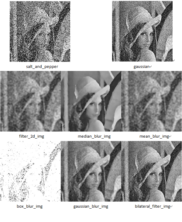
Image Filter Code Section:
import cv2
import numpy as np

salt_and_pepper_img=cv2.imread('salt_and_pepper.jpg')
gaussian_img=cv2.imread('gaussian.jpg')

#Two-dimensional convolution
kernel=np.ones((5,5),np.float32)/25
conv_2d_img=cv2.filter2D(salt_and_pepper_img,-1,kernel)
cv2.imwrite('filter_2d_img.jpg',conv_2d_img)

#median filtering
median_blur_img=cv2.medianBlur(salt_and_pepper_img,5)
cv2.imwrite('median_blur_img.jpg',median_blur_img)

#Mean filter
mean_blur_img=cv2.blur(salt_and_pepper_img,(5,5))
cv2.imwrite('mean_blur_img.jpg',mean_blur_img)

#box filter
box_blur_img=cv2.boxFilter(salt_and_pepper_img,-1,(2,2),normalize=False)
cv2.imwrite('box_blur_img.jpg',box_blur_img)

#Gauss filter
gaussian_blur_img=cv2.GaussianBlur(gaussian_img,(5,5),0)
cv2.imwrite('gaussian_blur_img.jpg',gaussian_blur_img)

#Bilateral filter
bilateral_filter_img=cv2.bilateralFilter(gaussian_img,9,75,75)
cv2.imwrite('bilateral_filter_img.jpg',bilateral_filter_img)

Gauss and bilateral filters the Gauss noise graph, and the rest filters the salt and pepper graph