According to Wu Enda's machine learning video, the gradient descent algorithm is learned and implemented by code.

The purpose of gradient descent algorithm is to find the value of theta, which minimizes the cost function, and to attach relevant formulas.

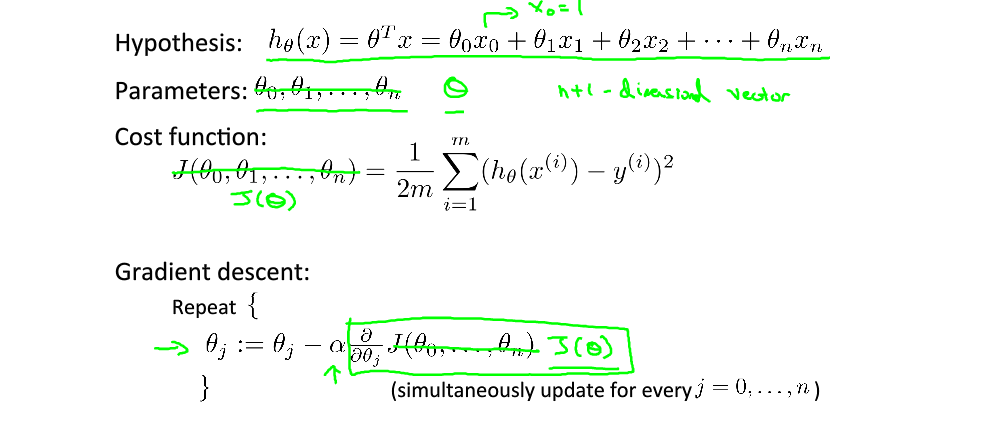
The above figure is the definition of hypothetical function and cost function, and the purpose of gradient descent algorithm is to find the lowest theta value of cost function. The formula of gradient descent algorithm is attached.

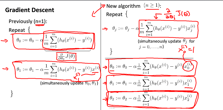
It should be noted that the gradient descent algorithm needs to update the value of theta at the same time.

Next, the algorithm is implemented by Wu Enda's gradient descent algorithm and an example to verify its correctness. The following code is implemented in Python

example1

Construct a set of scatter points (x,y), where x and y are linearly related y = k x + B (where k equals Tianhetan 1 and B equals theta 0). Calculate the value of K and b b y gradient descent algorithm.

import numpy as np
import matplotlib.pyplot as plt
import matplotlib

def computeCost(X, y, theta):
    m = len(y)
    J = np.sum(np.square(X.dot(theta) - y)) / (2 * m)
    return J


def gradientDescent(X, y, theta, alpha, num_iters):
    m = len(y)
    J_history = np.zeros((num_iters, 1))
    temp = theta
    # temp0 = theta[0,0]
    # temp1 = theta[1,0]
    for i in range(num_iters):
        for j in range(X.shape[1]):
            temp[j,0] = theta[j,0] - alpha / m * np.sum((X.dot(theta) - y) * X[:,j].reshape(50,1))
        # Method two
        # temp0 = theta[0,0] - alpha / m * np.sum((X.dot(theta) - y))
        # temp1 = theta[1,0] - alpha / m * np.sum((X.dot(theta) - y) * X[:,1].reshape(50,1))
        theta = temp
        # theta[0,0] = temp0
        # theta[1, 0] = temp1
        J_history[i] = computeCost(X, y, theta);

    return (theta,J_history)

#Suppose there are 50 samples.
matplotlib.rcParams['font.family'] = 'SimHei'
x_data = np.random.randint(1,50,(50,1))
y = 2.5 * x_data + 3
plt.plot(x_data,y,'r*',label = 'Scatter data')



X = np.hstack((np.ones((50,1)),x_data))
theta = np.array([[0.],[0.]])
iterations = 10000
alpha = 0.002
#Computational cost function
J = computeCost(X, y, theta);
print('J = {:0.2f}'.format(J))
#Running gradient descent algorithm
theta,J_history = gradientDescent(X, y, theta, alpha, iterations);
plt.plot(x_data,x_data * theta[1,0] + theta[0,0],label = 'y=theta0 + theta1 * X')
print(theta)
plt.legend()
plt.show()

The results of the above code are as follows:

J = 2943.36
[[2.98963149]
 [2.5002961 ]]

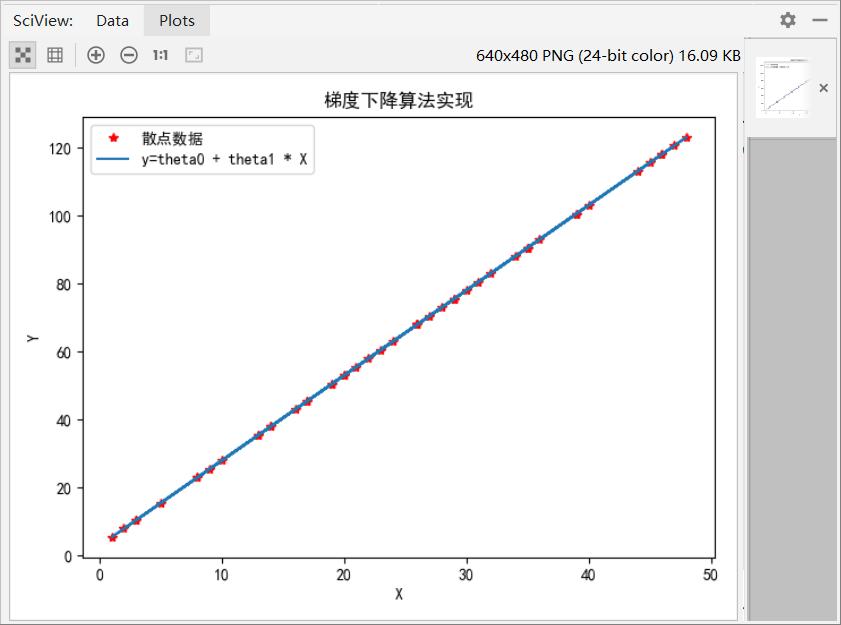
The effect is obvious. Gradient descent algorithm can fit scatter data very well, and the results are basically consistent with expectations.

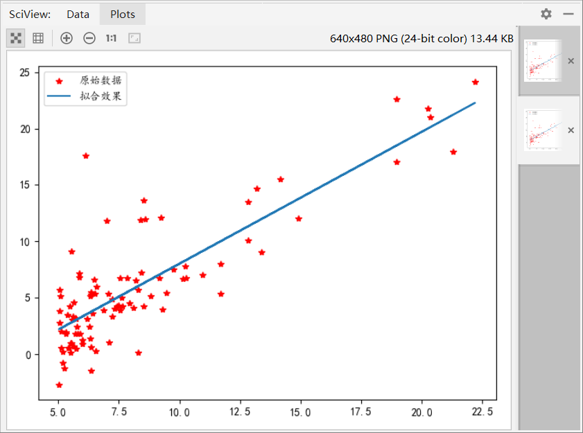
example2

Wu Enda Machine Learning Exercise, Single Variable Data Fitting Using Gradient Decline Algorithms

import numpy as np
import matplotlib.pyplot as plt
import matplotlib
# Computational cost function
def computeCost(X, y, theta):
    global  m
    J = np.sum(np.square(X.dot(theta) - y)) / (2 * m)
    return J

# Implementation of gradient descent algorithm
def gradientDescent(X, y, theta, alpha, iterations):
    global m
    temp = theta
    for iter in range(iterations):
        for i in range(X.shape[1]):
            temp[i,0] = theta[i,0] - alpha / m * (np.sum((X.dot(theta) - y) * X[:,i].reshape(m,1)))
        theta = temp
    return theta
#Data file path and read file
filepath = r'G:\MATLAB\machine-learning-ex1\ex1\ex1data1.txt'
data = np.loadtxt(filepath,delimiter=',')
#Constructing Matrix Based on Raw Data
matplotlib.rcParams['font.family'] = 'Kaiti'
X = data[:,0].reshape(len(data[:,0]),1)
y = data[:,1].reshape(len(data[:,1]),1)
plt.plot(X,y,'r*',label = 'Raw data')

m = len(y) #m samples
# Give constant 1 according to gradient descent algorithm x1
X = np.hstack((np.ones((m,1)),X))

# Calculating the Initial Cost Function
theta = np.zeros((2,1))
J = computeCost(X, y, theta)
print('theta = [[0],[0]]The value of the cost function is{:0.3f}'.format(J))

#Running gradient descent algorithm
iterations = 1500
alpha = 0.01
theta = gradientDescent(X, y, theta, alpha, iterations)
print('After running gradient descent algorithm theta0 = {:0.3f},theta1 = {:0.3f}'.format(theta[0,0],theta[1,0]))
plt.plot(data[:,0],theta[1,0] * data[:,0] + theta[0,0],label = 'Fitting effect')
plt.legend()
plt.show()

The results are as follows:

When theta = [[0],[0], the value of the cost function is 32.073
 After running gradient descent algorithm, theta 0 = 3.636, theta 1 = 1.167