preface

During this period of time, I have benefited a lot from watching the explanation of in-depth learning by up Master Liu Er of station b. Let me know what Inception is and how to embed the structure into the model. Here is the video address:

https://www.bilibili.com/video/BV1Y7411d7Ys?p=11&share_source=copy_web

Interested friends can also try to put the Inception structure into the code identified by mnist data before. Because the dimension changes, the parameters of the whole connection layer also need to be changed accordingly. The link is as follows:
https://blog.csdn.net/qq_42962681/article/details/116270125?spm=1001.2014.3001.5501

The following is the main body of this article for reference. If there are deficiencies, please correct them and learn together.

1, What is Inception?

When you build a convolution layer, you have to decide the size of the convolution kernel. How to judge which convolution kernel is better? Is 1x1 appropriate, 3x3 appropriate, or 5x5 appropriate? Do you want to add a pooling layer?
Since these parameters are super parameters and need to be set manually, it is undoubtedly a time-consuming and laborious project to try one by one in the experiment. At this time, the corresponding problems can be well solved through the Inception module.

Multiple different convolution kernels are used to process the input image at the same time (ensure that the output image size remains unchanged, only change its dimension), and finally splice the processed data.

2, Use steps

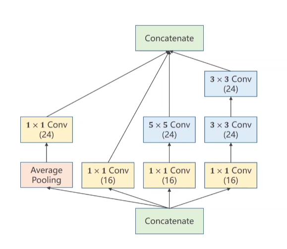
1. Spatial structure

The structure is shown in the figure (example):
In the figure, 5x5 convolution and 3x3 convolution fill the image accordingly, so the input image scale and output image scale remain unchanged.

2. Structural model

The code is as follows (example):
The data set in the code I use is the commonly used MNIST data set, and the sample size of a single image is (1, 28, 28).

Schematic diagram of inception code

import torch
import torch.nn as nn
from torch.utils.data import DataLoader  # We want to load the data set
from torchvision import transforms  # Raw data processing
from torchvision import datasets  # pytorch is very considerate to prepare this data set directly for us
import torch.nn.functional as F  # Activation function
import torch.optim as optim

#Inception of inception
#In the image input network, four different convolutions are processed at the same time. Here, it is ensured that the w and h processed respectively are the same for rear splicing
#The above data set [C = 64, b=64], which is directly mentioned here_ Size, which can be set freely.
class InceptionA(torch.nn.Module):
    def __init__(self,in_channels):
        super(InceptionA,self).__init__()
        #[64,1,28,28] - [64,16,28,28] through the convolution with one convolution kernel, the image size remains unchanged
        self.branch1x1 = nn.Conv2d(in_channels,16,kernel_size=1)

        self.branch5x5_1 = nn.Conv2d(in_channels, 16, kernel_size=1)
        # [64,16,28,28] - [64,24,28,28] through the convolution with convolution kernel of 5, because w and h are filled with 2 respectively, the image size remains unchanged
        self.branch5x5_2 = nn.Conv2d(16,24, kernel_size=5,padding=2)

        self.branch3x3_1 = nn.Conv2d(in_channels, 16, kernel_size=1)
        # [64,16,28,28] - [64,24,28,28] through the convolution with convolution kernel of 3, because 1 is filled, the image size remains unchanged
        self.branch3x3_2 = nn.Conv2d(16, 24, kernel_size=3, padding=1)
        # [64,24,28,28] - [64,24,28,28] through the convolution with convolution kernel of 3, because 1 is filled, the image size remains unchanged
        self.branch3x3_3 = nn.Conv2d(24, 24, kernel_size=3, padding=1)

        #[64,1,28,28]-[64,24,28,28]
        self.branch_pool = nn.Conv2d(in_channels, 24, kernel_size=1)

    def forward(self,x):
        branch1x1 = self.branch1x1(x)

        branch5x5 = self.branch5x5_1(x)
        branch5x5 = self.branch5x5_2(branch5x5)

        branch3x3 = self.branch3x3_1(x)
        branch3x3 = self.branch3x3_2(branch3x3)
        branch3x3 = self.branch3x3_3(branch3x3)

        #The average pool size remains unchanged
        branch_pool = F.avg_pool2d(x, kernel_size=3, stride=1, padding=1)
        branch_pool = self.branch_pool(branch_pool)

        outputs = [branch1x1, branch5x5, branch3x3, branch_pool]
        #[b,c,h,w] dim=1 is the dimension direction splicing. The returned dimension here is the sum of the above dimensions (16 + 24 + 24 + 24 = 88)
        return torch.cat(outputs, dim=1)

Module diagram

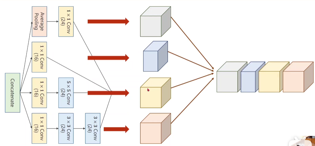
Through the pictures of inception, only the number of channels is changed without changing the size of the image. Therefore, the stitching is carried out in the dimension direction. The number of channels after stitching in the above figure is 24 + 16 + 24 + 24 = 88, which corresponds to the input dimension of the second layer of convolution layer below.

Embedding inception structure into our network

# Next, let's look at how the model is made
class Net(torch.nn.Module):
    def __init__(self):
        super(Net, self).__init__()
        # The first convolution layer we need to use is defined, because the image input channel is 1, and the first parameter is
        # The output channel is 10, kernel_size is the size of the convolution kernel, which is defined here as 5x5
        self.conv1 = torch.nn.Conv2d(1, 10, kernel_size=5)
        # You can understand the definition above, and you can understand it below
        self.conv2 = torch.nn.Conv2d(88, 20, kernel_size=5)

        #Call inception
        self.incep1 = InceptionA(in_channels=10)
        self.incep2 = InceptionA(in_channels=20)

        # Define another pooling layer
        self.mp = torch.nn.MaxPool2d(2)
        # Finally, the linear layer we use for classification
        self.fc = torch.nn.Linear(1408, 10)

    # The following is the calculation process
    def forward(self, x):
        # Flatten data from (n, 1, 28, 28)
        batch_size = x.size(0)  # 0 here is the first parameter of x size, which automatically obtains the batch size
        #(64, 1, 28, 28) after convolution of 10 groups of kernel=5 ((64, 10, 24, 24)), through maximum pooling (64, 10, 12, 12)
        x = F.relu(self.mp(self.conv1(x)))
        # Input to inception (64, 10, 12, 12), the size remains unchanged, and the dimensions are added (64, 88, 12, 12)
        x = self.incep1(x)
        # (64, 88, 12, 12) after convolution of 20 groups of kernel=5 ((64, 20, 8, 8)), through maximum pooling (64, 20, 4, 4)
        x = F.relu((self.mp(self.conv2(x))))
        #Input to inception (64, 20, 4, 4), the size remains unchanged, and the dimensions are added (64, 88, 4, 4) ioriw
        x = self.incep2(x)
        # In order to give us the last fully connected linear layer
        # We want to change a two-dimensional picture (actually, it has been processed here) 64x88x4 tensor into one-dimensional
        x = x.view(batch_size, -1)  # flatten
        #64x88x4 changed to 64x1408
        # Through the linear layer, determine the probability that it is 0 ~ 9 each number
        #64x1408 changed to 64x10 because the handwritten data set has 10 categories
        x = self.fc(x)
        return x

summary

There is no end to learning. The more you go on, the more you find that you don't understand. You feel small and need to continue to work hard.