1, Introduction

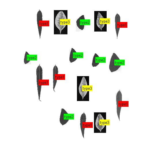
This topic is a leaf recognition system based on MATLAB HU moment invariants. By calculating the geometric characteristics of various leaves, we can judge what type of leaves they belong to.
Geometric moment was proposed by Hu(Visual pattern recognition by moment invariants) in 1962. It has translation, rotation and scale invariance.


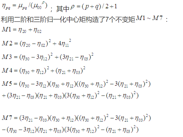
These seven invariant moments form a set of characteristic quantities, Hu M. K proved that they are invariant to rotation, scaling and translation in 1962.
In fact, in the process of object recognition in the picture, only the and invariance are maintained well, and the errors caused by other invariant moments are relatively large. Some scholars believe that only the invariant moment based on the second-order moment can describe the two-dimensional object with rotation, scaling and translation invariance (and just consist of the second-order moment). But I didn't prove whether it was true.
The feature quantity composed of Hu moment has the advantage of fast speed, but the disadvantage is that the recognition rate is relatively low. I have done gesture recognition. For the segmented gesture contour map, the recognition rate is about 30%, and for the pictures with rich texture, the recognition rate is even less eye-catching, only about 10%. This is partly because Hu moment invariants only use low-order moments (at most, third-order moments), and the details of the image are not well described, resulting in the incomplete description of the image.
Hu moment invariants are generally used to identify large objects in the image. The shape of the object is well described, and the texture features of the image cannot be too complex. For example, the recognition effect of fruit shape or simple characters in the license plate will be relatively better.
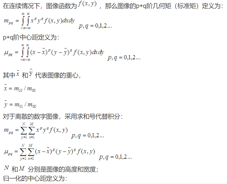
It is defined as follows:
① Definition of moment invariants of order (p+q):
② For digital images, discretization is defined as:
③ Definition of normalized central moment:
④ Hu moment definition

2, Source code

close all
clear all
clc
tic
f=imread('test.tif');%Read in test chart
A=double(f);%Convert gray value to double precision
g=mat2gray(A);%The gray value is normalized between 0 and 1
k=im2bw(g,0.4);%Binarization, threshold 0.4
 imshow(k);
k=1-k;%reversal

se=strel('disk',6);
fc=imclose(k,se);%Closed operation
fc=imfill(fc,'hole');%Hole filling

figure,imshow(fc);
se=strel('disk',8);
fco=imopen(fc,se);%Open operation
figure,imshow(fco);

BW=fco;
trainset=train(); 
trainset2=train2();%training sample 
imshow(f,[]);
[L,num] = bwlabel(BW); %sign
for t=1:num
    [r c]=find(L==t);
    r1=min(r);
    c1=min(c);
    r2=max(r);
    c2=max(c);
    IM{t}=BW(r1:r2,c1:c2);

%          figure;imshow(BW(r1:r2,c1:c2))
    phi=invmoments(IM{t});  %Extracting moment invariant features
    Pset{t}=phi; 
    d(t)=norm(abs(log(Pset{t}(1:7)))-abs(log(trainset(1:7)))); %Match with training samples
d2(t)=norm(abs(log(Pset{t}(1:7)))-abs(log(trainset2(1:7))));
  
 
end
function [trainset]= train( )
%TRAIN Summary of this function goes here
%   Detailed explanation goes here

     f= imread('train_1.tif');
 A=double(f);
g=mat2gray(A);
k=im2bw(g,0.4);

k=1-k;
se=strel('disk',6);
fc=imclose(k,se);
fc=imfill(fc,'hole');

se=strel('disk',15);
fco=imopen(fc,se);
%BW=im2bw(I,0.001);
%BW=imfill(BW,'hole'); 
%SE=strel('disk',10);
%BW=imopen(BW,SE);
% figure;imshow(BW);
BW=fco;
[r c]=find(BW==1);
    r1=min(r);
    c1=min(c);
    r2=max(r);
    c2=max(c);
    function phi = invmoments(F)
%INVMOMENTS Compute invariant moments of image.
%   PHI = INVMOMENTS(F) computes the moment invariants of the image
%   F. PHI is a seven-element row vector containing the moment
%   invariants as defined in equations (11.3-17) through (11.3-23) of
%   Gonzalez and Woods, Digital Image Processing, 2nd Ed.
%
%   F must be a 2-D, real, nonsparse, numeric or logical matrix.

%   Copyright 2002-2004 R. C. Gonzalez, R. E. Woods, & S. L. Eddins
%   Digital Image Processing Using MATLAB, Prentice-Hall, 2004
%   $Revision: 1.5 $  $Date: 2003/11/21 14:39:19 $

if (ndims(F) ~= 2) | issparse(F) | ~isreal(F) | ~(isnumeric(F) | ...
                                                    islogical(F))
   error(['F must be a 2-D, real, nonsparse, numeric or logical ' ...
          'matrix.']); 
end

F = double(F);

phi = compute_phi(compute_eta(compute_m(F)));
  
%-------------------------------------------------------------------%
function m = compute_m(F)

[M, N] = size(F);
[x, y] = meshgrid(1:N, 1:M);
  
% Turn x, y, and F into column vectors to make the summations a bit
% easier to compute in the following.
x = x(:);
y = y(:);
F = F(:);
  
% DIP equation (11.3-12)
m.m00 = sum(F);
% Protect against divide-by-zero warnings.
if (m.m00 == 0)
   m.m00 = eps;
end

3, Operation results

4, Remarks

Complete code or write on behalf of QQ 912100926