git official link: GitHub - facebookresearch/mae: PyTorch implementation of MAE https//arxiv.org/abs/2111.06377

I can't understand the MAE code at all. I want to understand this code step by step. I think it's useful to see the great God code. This article is for notes.

1, Running example:

How to say, it must be taking out the code in the demo for a run. But there will be problems. The following is the code for the demo. The first question is

TypeError: __init__() got an unexpected keyword argument 'qk_scale'

It's easy to say that the function doesn't have this parameter. Find the position and delete it. I dare to delete it because its value is None. Just delete it directly

The second problem is that I put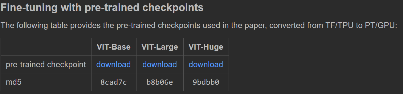

These three models are regarded as pre training models, and the results are shown on the left below, which restores loneliness. After thinking about whether kaiming was wrong for a long time and how kaiming could be wrong for a long time, I found that the pre training model was hidden in the link. The following three are just the pre training models he used when he started training.

 

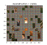
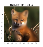
Link to find the two large model parameters in the demo. The results of the run are as follows. Right

https://dl.fbaipublicfiles.com/mae/visualize/mae_visualize_vit_large.pth

https://dl.fbaipublicfiles.com/mae/visualize/mae_visualize_vit_large_ganloss.pth

The replay is over (bushi)

Finally got the demo through.

2 drawing

It's amazing to debug this method. We got through the demo. Let's follow the demo to see the full picture of the model!

This section obtains the image and normalizes it ， and then draws it with plt ， here is to normalize the drawing first and then return to it.  

Make an unnecessary move to make complaints about it. (Tucao: I don't understand why I want to normalize first and come back to paint again. What I do is show img is not fragrant?)

# load an image
img_url = 'https://user-images.githubusercontent.com/11435359/147738734-196fd92f-9260-48d5-ba7e-bf103d29364d.jpg' # fox, from ILSVRC2012_val_00046145
# img_url = 'https://user-images.githubusercontent.com/11435359/147743081-0428eecf-89e5-4e07-8da5-a30fd73cc0ba.jpg' # cucumber, from ILSVRC2012_val_00047851
img = Image.open(requests.get(img_url, stream=True).raw)
#raw is a kind of format, stream is to make sure that it can go down and down again. (for example, memory will be determined in advance)
img = img.resize((224, 224))
img = np.array(img) / 255.

assert img.shape == (224, 224, 3)

# normalize by ImageNet mean and std
img = img - imagenet_mean
img = img / imagenet_std

plt.rcParams['figure.figsize'] = [5, 5]   #Set canvas size
show_image(torch.tensor(img))

def show_image(image, title=''):
    # image is [H, W, 3]
    assert image.shape[2] == 3
    plt.imshow(torch.clip((image * imagenet_std + imagenet_mean) * 255, 0, 255).int())
    #Just normalized, now return, remember clip to prevent crossing the boundary, int to prevent decimals, because pixels are integers, imshow can even read tensors
    plt.title(title, fontsize=16)
    plt.show()
    plt.axis('off')
    return

3 load model

3.1 model preparation

chkpt_dir = 'model_save/mae_visualize_vit_large.pth'
model_mae = prepare_model(chkpt_dir, 'mae_vit_large_patch16')
print('Model loaded.')

It will enter the function of preparing the model

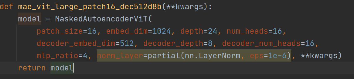
def prepare_model(chkpt_dir, arch='mae_vit_large_patch16'):
    # build model
    model = getattr(models_mae, arch)()
    # load model
    checkpoint = torch.load(chkpt_dir, map_location='cpu')
    msg = model.load_state_dict(checkpoint['model'], strict=False)
    print(msg)

    return model

For the first game getattr(models_mae,arch): Yes, take models_ The arch in the MAE module # and what is this arch? As can be seen in the figure below, it is a function without parentheses (I don't understand), so a parenthesis should be added after get

        

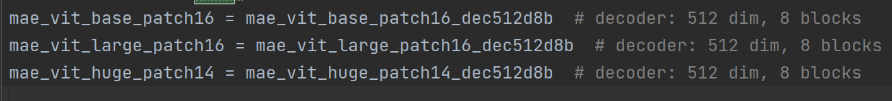
Then we enter this function and we can see this function. Oh ~ it is a function to obtain the model. There are three different functions in large, medium and small models. The parameters of different functions are different.

Then there is a big project. Let's take a look inside the model.

3.2.1_ Inside the model

If the model code is too large, I won't paste the whole one. I paste it part by part.

3.2.1.1 # encoder module

from timm.models.vision_transformer import PatchEmbed, Block


self.patch_embed = PatchEmbed(img_size, patch_size, in_chans, embed_dim)
#patch_size should be the size of a picture. inchans are usually three picture layers
# Embedded -- dim is a feature dimension compiled


num_patches = self.patch_embed.num_patches
##num_ The size of pathches is x*y, which means that the picture is divided into x*y parts num_patches = (224/patch_size)**2 = 14 **2 = 196

This code comes from the code of VIT, but I haven't seen what the code of VIT looks like. I won't write it in this article until the next article. I'll traverse into this coding function to see what it is. Let's remember that there is a coding function. It seems that the picture becomes a string of feature codes

self.cls_token = nn.Parameter(torch.zeros(1, 1, embed_dim))
self.pos_embed = nn.Parameter(torch.zeros(1, num_patches + 1, embed_dim),         
    requires_grad=False)  # fixed sin-cos embedding

CLS token join location code {NN The function of patameter is to convert an untrained tensor or matrix into parameters that can be trained in the model. (I want to write a parameter to be trained, but it's not the official layer. I finally know the method.). cls_ The token size is (1, 11024) and the location code is (11971024). Why is 197? It should be to keep consistent with the code size after embedding CLS, and then cat# I guess.

        self.blocks = nn.ModuleList([
            Block(embed_dim, num_heads, mlp_ratio, qkv_bias=True, norm_layer=norm_layer)
            for i in range(depth)])
        self.norm = norm_layer(embed_dim)

The block here is the one in the VIT. This block will be discussed when the vit code

Here are some little trick s they use

        

nn.LayerNorm   #This representation is normalized on the channel 
nn.batchNorm  #This is normalized on batch
DropPath  # This is also a drop method different from dropout
nn.GELU   #An activation function 

nn.ModuleList is actually a list. Put some blocks in this list. Unlike ordinary lists, ordinary lists will not be trained. Here are 24 self attention blocks, each with 12 heads. The above is the module used by the encoder.

3.2.1.2 decoding module

Here is the decoder.  

        self.decoder_embed = nn.Linear(embed_dim, decoder_embed_dim, bias=True)
            # One fc layer 1024 to 512

        self.mask_token = nn.Parameter(torch.zeros(1, 1, decoder_embed_dim))
            #One mask code (1, 1512)
        self.decoder_pos_embed = nn.Parameter(torch.zeros(1, num_patches + 1,         
            decoder_embed_dim), requires_grad=False)  # fixed  sin-cos embedding
              #A location code and no training (1197512) why not training?
        

        self.decoder_blocks = nn.ModuleList([
            Block(decoder_embed_dim, decoder_num_heads, mlp_ratio, qkv_bias=True, norm_layer=norm_layer)
            for i in range(decoder_depth)])

        self.decoder_norm = norm_layer(decoder_embed_dim)

        self.decoder_pred = nn.Linear(decoder_embed_dim, patch_size**2 * in_chans, bias=True) # decoder to patch
        #Prediction layer 512 to 256 * 3 (this is less than 224 * 224 * 3)

The attention layer of the decoder has only 8 layers, but it is also 12 heads. The input is 512 dimensions

3.2.1.3 initialization module

3.2.1.3.1 location code

        self.norm_pix_loss = norm_pix_loss

        self.initialize_weights()

The value of the first one is false. We'll see what's useful later. The second one is a function. Let's go in and have a look.

       pos_embed = get_2d_sincos_pos_embed(self.pos_embed.shape[-1], int(self.patch_embed.num_patches**.5), cls_token=True)
        self.pos_embed.data.copy_(torch.from_numpy(pos_embed).float().unsqueeze(0))

The first step of initialization is a location coding function. Let's enter this coding function to see

def get_2d_sincos_pos_embed(embed_dim, grid_size, cls_token=False):  
    #embed_dim = 1024 is the last dimension of the position, and gridSize is the length and width of each small patch, that is, 14
    
  
    grid_h = np.arange(grid_size, dtype=np.float32)
    grid_w = np.arange(grid_size, dtype=np.float32)
      #Generate two coordinate systems 14 * 14 


    grid = np.meshgrid(grid_w, grid_h)  # here w goes first
    #This is a coordinate system, but we need to see who is x and who is y 
    grid = np.stack(grid, axis=0)
    #  Two meshes are generated. Each is 14 * 14 grid, and now it is (2,14,14)


    grid = grid.reshape([2, 1, grid_size, grid_size])  
    #(2,1,14,14)


   

Then continue to enter the lower function, we continue to see.

    pos_embed = get_2d_sincos_pos_embed_from_grid(embed_dim, grid)


def get_2d_sincos_pos_embed_from_grid(embed_dim, grid):
    assert embed_dim % 2 == 0

    # use half of dimensions to encode grid_h
    emb_h = get_1d_sincos_pos_embed_from_grid(embed_dim // 2, grid[0])  # (H*W, D/2)
    emb_w = get_1d_sincos_pos_embed_from_grid(embed_dim // 2, grid[1])  # (H*W, D/2)

    emb = np.concatenate([emb_h, emb_w], axis=1) # (H*W, D)
    return emb

Then enter the lower function.

def get_1d_sincos_pos_embed_from_grid(embed_dim, pos):

    

    """
    embed_dim: output dimension for each position   There are only 512 here
    pos: a list of positions to be encoded: size (M,)    #Here is (1, 14, 14) equivalent to a channel
    out: (M, D)
    """
    assert embed_dim % 2 == 0
    omega = np.arange(embed_dim // 2, dtype=np.float)
    #    (1，2，3，4.. . . 256)
    omega /= embed_dim / 2.
    #This step is normalization

    omega = 1. / 10000**omega  # (D/2,)
    ##It's a bit like doing a reverse. It used to be 0 to 1, but now it's 1 to 0

    pos = pos.reshape(-1)  # (M,)
    #1, 14 and 14 become 196 forms, which are 0 to 13 cycles 14 times 
    out = np.einsum('m,d->md', pos, omega)  # (M, D/2), outer product
        #Here is the outer set, that is, multiplying a column by a row is equivalent to out and becomes a matrix of (196256).

    emb_sin = np.sin(out) # (M, D/2)
    emb_cos = np.cos(out) # (M, D/2)
    
    emb = np.concatenate([emb_sin, emb_cos], axis=1)  # (M, D)

    #After taking sin and cos for all values, con is added, but note that the dimension is 1, that is, the first half of 196 * 512 is sin and the second half of cos
    return emb

After the lower level function returns, it is spelled into 196 * 1024 again. This location code is really hard. Let's see how he came. First, 1961024 is divided into two sections. Look at the first half. First make a (256,1) long matrix distribution, then 1256 represents the position, and then reverse it and make an outer product with the value leveled with the grid (14 * 14). This grid is also the position information. After that, two position codes are obtained on both sin and cos. Then put it together to get a dimension code. Then put the two dimensions together to get the overall position code.  

    if cls_token:
        pos_embed = np.concatenate([np.zeros([1, embed_dim]), pos_embed], axis=0)
    return pos_embed

Here is the one dimension of CLS by changing 196 1041 into (1971024).

3.2.1.3.2 return to initialization

        self.pos_embed.data.copy_(torch.from_numpy(pos_embed).float().unsqueeze(0))
        #The position code of the encoder is obtained by changing numpy into tensor, then turning to float32 and expanding the dimension to (11971024)

  decoder_pos_embed = get_2d_sincos_pos_embed(self.decoder_pos_embed.shape[-1], int(self.patch_embed.num_patches**.5), cls_token=True)
        self.decoder_pos_embed.data.copy_(torch.from_numpy(decoder_pos_embed).float().unsqueeze(0))

The position coding (1197512) of the decoder is still half less than that of the encoder

        w = self.patch_embed.proj.weight.data
        torch.nn.init.xavier_uniform_(w.view([w.shape[0], -1]))


        torch.nn.init.normal_(self.cls_token, std=.02)
        torch.nn.init.normal_(self.mask_token, std=.02)

This w is the weight value of the weight layer. It can be seen that the size of W is (1024, 3, 16, 16). 1024 is the output dimension and 3 is the input dimension. Equivalent to a convolution? Then the parameters are initialized and unified in the (1024, 3 * 16 * 16) positive distribution

mask and cls should also be initialized.

        

self.apply(self._init_weights)

Initialize other layers self Apply should use the following function for each module of the traversal model. Let's enter the initialization weight function to have a look,

    def _init_weights(self, m):
        if isinstance(m, nn.Linear):
            # we use xavier_uniform following official JAX ViT:
            torch.nn.init.xavier_uniform_(m.weight)
            if isinstance(m, nn.Linear) and m.bias is not None:
                nn.init.constant_(m.bias, 0)
        elif isinstance(m, nn.LayerNorm):
            nn.init.constant_(m.bias, 0)
            nn.init.constant_(m.weight, 1.0)

You can see how to initialize the weight of the full connection layer, use xavier's uniform distribution, and set the bias to 0

The offset of layer normalization layer is 0 and the weight is 1

During the process, we can see that 24 attention layers are initialized, and there are various linear layers in the attention layer.

3.2.1.3.3 initialization completed

So far, the initialization of the model is completed, and we have obtained the model. From these steps, we can roughly see what the model looks like. There is an encoder module and a decoder module. The encoder module has a 24 layer deep 16 head self attention module. There are also some location coding and cls coding, but the decoder only has one more mask coding, and the dimension will be different from that of the encoder.

3.3 model preparation is completed.  

checkpoint = torch.load(chkpt_dir, map_location='cpu')

This chkpt_dir, that is, the downloaded pre training model should probably be only parameters, so you need to load parameters in the following sentence

This strict here means that if there are layers with pre training, the pre training parameters will be used, and the layers without pre training in the model will be initialized normally.  

msg = model.load_state_dict(checkpoint['model'], strict=False)

return model

msg records the loading results and {gets the whole model.

4 processing pictures

The model is ready. Let's start processing a picture with the model and have a look.  

4.1 data preparation

torch.manual_seed(2)   #Fixed random number seed
print('MAE with pixel reconstruction:')
run_one_image(img, model_mae)

We entered run_ONE_image function internal

    x = torch.tensor(img)

    # make it a batch-like
    x = x.unsqueeze(dim=0)
    x = torch.einsum('nhwc->nchw', x)

Here is how to make a picture into a batch. The third einsum can also be used

torch. The function of transfer () is a dimension conversion. Bring that 3 to the second dimension. But he they're really smart guys.

    loss, y, mask = model(x.float(), mask_ratio=0.75)

Enter the model and run it. The predicted value of loss and mask are returned from the model. Let's look inside the model. Note that the calculated values in the model are in float32 format.  

latent, mask, ids_restore = self.forward_encoder(imgs, mask_ratio)

The first sentence of forward is this sentence. Let's go into the forward encoder and have a look.  

4.2 coding steps

    def forward_encoder(self, x, mask_ratio):    
        # embed patches

        x = self.patch_embed(x)  #x: (1,322424) - > (11961024) 14 * 14 chip codes

        # add pos embed w/o cls token
        x = x + self.pos_embed[:, 1:, :] # pos is 11971024. The cls location information without 0 is directly added to the chip code. It's very different from my idea. Will it really work.

        # masking: length -> length * mask_ratio
        x, mask, ids_restore = self.random_masking(x, mask_ratio)
        

    def random_masking(self, x, mask_ratio):
        """
        Perform per-sample random masking by per-sample shuffling.
        Per-sample shuffling is done by argsort random noise.
        x: [N, L, D], sequence
        """
        N, L, D = x.shape  # batch, length, dim
        len_keep = int(L * (1 - mask_ratio))  #Calculate how many pieces need to be left
        
        noise = torch.rand(N, L, device=x.device)  # noise in [0, 1] noise(1，196)
        
        # sort noise for each sample
        ids_shuffle = torch.argsort(noise, dim=1)  # ascend: small is keep, large is remove
        # IDS sorts the value of noise_ Shuffle gets the subscript value.

        ids_restore = torch.argsort(ids_shuffle, dim=1)  #Reorder the subscripts obtained after sorting? This step#I don't understand the back 
        # keep the first subset
        ids_keep = ids_shuffle[:, :len_keep]    #Keep the noise level low?
        x_masked = torch.gather(x, dim=1, index=ids_keep.unsqueeze(-1).repeat(1, 1, D))
#This gather is the number of index es picked in the dim dimension of x. But curiously, isn't this a random selection?
# The dimension of index is (1, 491024) x and (11961024) x_masked is (1, 491024)

        # generate the binary mask: 0 is keep, 1 is remove
        mask = torch.ones([N, L], device=x.device)
        mask[:, :len_keep] = 0
        #mask is (1196), where the first 49 are all 0 and the following are all 1 
        
        # unshuffle to get the binary mask
        mask = torch.gather(mask, dim=1, index=ids_restore)
        #I finally understand this here ids_REStore The function of is to mask regard as noise Then put mask according to#The resulting mask is a two-dimensional tensor with 1 where there is a mask and 0 where there is no mask.

        return x_masked, mask, ids_restore

The mask here is very difficult to understand, so let me give an example.  

First, noise is generated randomly. For example, noise = [2,0,3,1]

Then sort argsort: shuffle = [1,3,0,2] here is to generate random numbers. We take the first two, that is, random 1,3, as the subscript of the mask

Sort shuffle: restore = [2, 0, 3, 1]

mask = [0,0,1,1] we get [1,0,1,0] subscript 1 by retrieving the mask according to restore, and three places are 0 In fact, you can regard mask and shuffle as the same. You can use restore to retrieve the shuffle and get [0, 1, 2, 3] and find that they are sorted well. Access [1, 0, 1, 0] and get [0,0,1,1] which correspond to each other.

Handling cls

        cls_token = self.cls_token + self.pos_embed[:, :1, :]
        #cls plus location information 
        cls_tokens = cls_token.expand(x.shape[0], -1, -1)
          # This sentence is to prevent bulk copy, that is, extended copy. If the batch of x is n CLS, N copies should also be copied


        x = torch.cat((cls_tokens, x), dim=1)

        #x: (1,501024) - > (1,501024) was originally expanded in the one dimension of the number of slices.

Here x we have to go through the training of 24 multi head self attention, and then normalize.

        for blk in self.blocks:
            x = blk(x)
        x = self.norm(x)

4.3 decoding steps

Return to forward and come to the second game of decoding

pred = self.forward_decoder(latent, ids_restore)  # [N, L, p*p*3]

    def forward_decoder(self, x, ids_restore):
        # embed tokens
        x = self.decoder_embed(x)

        #x  (1,50,1024) ->(1,50,512)
        
        # append mask tokens to sequence
        mask_tokens = self.mask_token.repeat(x.shape[0], ids_restore.shape[1] + 1 - x.shape[1], 1)
        
        ##ids_restore.shape[1] + 1 - x.shape[1] =196+1-50 =147, that is, the number of cls pieces minus x = the number of covers required
        #self. maskroken. shape = (1,1,512)  mask_ Tokens = (1147512) copy as many copies as you want

        x_ = torch.cat([x[:, 1:, :], mask_tokens], dim=1)  # no cls token cls worked hard all his life 
         #That's it. I haven't seen your role yet. Please wait a long time. Here is the X after completing the splicing of X and mask_


        x_ = torch.gather(x_, dim=1, index=ids_restore.unsqueeze(-1).repeat(1, 1, x.shape[2]))  # unshuffle is sorted by mask index shape = (1,196,512)
        x = torch.cat([x[:, :1, :], x_], dim=1)  # append cls token speechless

        # add pos embed
        x = x + self.decoder_pos_embed 

        # apply Transformer blocks
        for blk in self.decoder_blocks:
            x = blk(x)           
        x = self.decoder_norm(x)     #Just eight poor 

        # predictor projection
        x = self.decoder_pred(x)
        #### x (1,197.512) -> (1,197,768)


        # Remove CLS token CLS: there's something wrong with you, isn't it. 
        x = x[:, 1:, :]

        return x

The image results predicted by the model are obtained

4.4 loss exploration

The next step is loss

        pred = self.forward_decoder(latent, ids_restore)  # [N, L, p*p*3]
        loss = self.forward_loss(imgs, pred, mask)

        target = self.patchify(imgs)

First, enter this function, p is the size of a small graph, hw is the number of graphs in the yx direction, and p is 14

    def patchify(self, imgs):
        """
        imgs: (N, 3, H, W)
        x: (N, L, patch_size**2 *3)
        """
        p = self.patch_embed.patch_size[0]
        assert imgs.shape[2] == imgs.shape[3] and imgs.shape[2] % p == 0

        h = w = imgs.shape[2] // p
        x = imgs.reshape(shape=(imgs.shape[0], 3, h, p, w, p))
        x = torch.einsum('nchpwq->nhwpqc', x)
        x = x.reshape(shape=(imgs.shape[0], h * w, p**2 * 3))
        return x

x is (1, 3, 14, 16, 14, 16) - (1, 14, 14, 16, 16, 3)

Then reshape (1, 14, 14, 16, 16, 3) - (1196768) the process is not external. Who knows how you changed.

target = self.patchify(imgs) is to edit the original picture to the size of (1196768) 

        if self.norm_pix_loss:
            mean = target.mean(dim=-1, keepdim=True)
            var = target.var(dim=-1, keepdim=True)
            target = (target - mean) / (var + 1.e-6)**.5

This one didn't go in

Maybe it's because it's already gone

        loss = (pred - target) ** 2
        loss = loss.mean(dim=-1)  # [N, L], mean loss per patch

Loss is the square of the pixel difference, and then the average of the last dimension becomes (1196), that is, each small pat has a loss

        loss = (loss * mask).sum() / mask.sum()  # mean loss on removed patches
        return loss

The mask is 0 in the corresponding uncovered area, so it is only in the covered area that the loss is calculated and the loss value is returned. Back to run

4.5 drawing

    loss, y, mask = model(x.float(), mask_ratio=0.75)
    y = model.unpatchify(y)

According to the name, patch is restored to a large picture.

    def unpatchify(self, x):
        """
        x: (N, L, patch_size**2 *3)
        imgs: (N, 3, H, W)
        """
        p = self.patch_embed.patch_size[0]
        h = w = int(x.shape[1]**.5)
        assert h * w == x.shape[1]
        
        x = x.reshape(shape=(x.shape[0], h, w, p, p, 3))
        x = torch.einsum('nhwpqc->nchpwq', x)
        imgs = x.reshape(shape=(x.shape[0], 3, h * p, h * p))
        return imgs

p 16 h w, 14,14   

x (1,196,768) -> (1,14,14,16,16,3) ->(1,3,14,16,14,16)  ->imgs(1,3,224,224) 

#I suddenly figured out that there is no need to know how it changes here. I just need to be consistent. The computer will correspond them without taking care of them.  

Come back up there

    loss, y, mask = model(x.float(), mask_ratio=0.75)
    y = model.unpatchify(y)
    y = torch.einsum('nchw->nhwc', y).detach().cpu()

y(1，3，224，224)- >(1，224，224，3)

    # visualize the mask
    mask = mask.detach()
    mask = mask.unsqueeze(-1).repeat(1, 1, model.patch_embed.patch_size[0]**2 *3)  # (N, H*W, p*p*3)
    mask = model.unpatchify(mask)  # 1 is removing, 0 is keeping
    mask = torch.einsum('nchw->nhwc', mask).detach().cpu()

mask:(1,196 )  ->(1,196,768) ->(1,3,224,224)  ->(1,224,224,3) 

    x = torch.einsum('nchw->nhwc', x)

    # masked image
    im_masked = x * (1 - mask)

    # MAE reconstruction pasted with visible patches
    im_paste = x * (1 - mask) + y * mask

x (1,3,224,224) ->(1,224,224,3)

1-mask ， is the original 0, which is not covered, becomes 1, and the covered becomes 0 multiplied by x to get the covered picture.

im_paste = x * (1 - mask) + y * mask * the picture covered plus the predicted Y multiplied by the mask. Because the mask covers 1, it is multiplied directly

So far, all the images that need to be drawn are obtained.,  

    # make the plt figure larger
    plt.rcParams['figure.figsize'] = [24, 24]

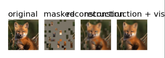
    plt.subplot(1, 4, 1)
    show_image(x[0], "original")

    plt.subplot(1, 4, 2)
    show_image(im_masked[0], "masked")

    plt.subplot(1, 4, 3)
    show_image(y[0], "reconstruction")

    plt.subplot(1, 4, 4)
    show_image(im_paste[0], "reconstruction + visible")

    plt.show()

Why didn't the picture come out together????

 

It was because I changed the code

 

ok, it's over. The demonstration is over. Look at other modules another day