Overview of whale optimization algorithm

Whale Optimization Algorithm (WOA) is a meta heuristic algorithm based on humpback whale hunting method proposed by Mirjalili in 2016. It has been successfully applied to various complex discrete optimization problems, such as resource scheduling problem, construction site workflow planning, location and path planning, neural network training and so on. In terms of algorithm improvement and application, Yan Xu et al. Proposed a hybrid stochastic quantum Whale Optimization Algorithm to solve TSP problem; Teng Deyun and others improved Whale Optimization Algorithm by combining Whale Optimization Algorithm with topology to solve multi-objective reactive power optimization scheduling problem; Tu Chunmei et al. Proposed chaotic feedback adaptive optimization algorithm; Liu zhusong et al. Proposed positive co chaotic double string optimization algorithm (CSCWOA); Zhong Minghui et al. Proposed an efficient optimization algorithm for randomly adjusting control parameters

WOA

WOA can be used to solve continuity optimization problems. Therefore, by investigating the express delivery situation of several express companies in Jinzhou City, it is found that customer satisfaction and distribution efficiency are not ideal, mainly because each customer point has different time periods for receiving express mail, resulting in the back and forth of couriers and unnecessary time waiting, which not only greatly reduces the distribution efficiency of couriers, At the same time, it also greatly reduces customer satisfaction. Therefore, this paper introduces the greedy exchange mechanism into the whale optimization algorithm, establishes the express terminal distribution path model with time window based on the greedy whale optimization algorithm (GWOA), and solves the example. The results show that GWOA has better convergence speed and better local optimization ability.

Express terminal distribution

Description of routing problem the express terminal distribution routing problem can be described as: the courier starts from the distribution center (express distribution network), sends the customer's goods to each customer point along a specific route, and then needs to return to the starting point (express distribution network point) before a fixed time. During this period, couriers can choose short distance and time-saving routes to complete express delivery according to their own experience, or give priority to some customers according to their special needs. The premise is to ensure that all customer points are served before the specified time and can only be served once. Therefore, the express terminal distribution path should be reasonably planned to achieve the shortest distribution time, shortest distribution route distance, lowest distribution cost and maximum customer satisfaction under the constraints of meeting customer time window, customer demand, load limit of distribution vehicles and maximum driving distance of express vehicles.

tic
clear
clc
%% use importdata This function reads the file
data=importdata('input.txt');
cap=160;
%% Extract data information
vertexs=data(:,2:3);                %Coordinates of all points x and y
customer=vertexs(2:end,:);          %Customer coordinates
cusnum=size(customer,1);            %Number of customers
v_num=3;                            %Initial number of vehicles used
demands=data(2:end,4);              %requirement
h=pdist(vertexs);
dist=squareform(h);                 %Distance matrix
%% Whale optimization algorithm parameters
NIND=100;                           %Population number
MAXGEN=300;                         %Maximum number of iterations
N=cusnum+v_num-1;                   %Whale individual length=Number of customers+Maximum number of vehicles used-1
belta=10;                           %Penalty function coefficient for violation of load constraint
%% Population initialization
init_vc=init(cusnum,demands,cap,dist);          %structure OVRP Initial solution
population=init_pop(NIND,N,cusnum,init_vc);
%% Route and total distance of output random solution
obj=obj_function(population,cusnum,cap,demands,dist,belta);
[min_obj,min_index]=min(obj);
disp('Optimal individual in initial population:')
[currVC,NV,TD,violate_num,violate_cus]=decode(population(min_index,:),cusnum,cap,demands,dist);       %Initial decoding
disp(['Number of vehicles used:',num2str(NV),'，Total vehicle distance:',num2str(TD),'，Number of constraint violation paths:',num2str(violate_num),'，Number of customers violating constraints:',num2str(violate_cus)]);
disp('~~~~~~~~~~~~~~~~~~~~~~~~~~~~~~~~~~~~~~~~~~~~~~~~~~~~~~~~~~~~~~~~')
%% Main cycle
gen=1;                              %Counter initialization
bestInd=population(min_index,:);    %Initialize global optimal individual
bestObj=min_obj;                    %Initial global optimal individual objective function value
BestPop=zeros(MAXGEN,N);            %Record the global optimal individual in each iteration
BestObj=zeros(MAXGEN,1);            %Record the objective function value of the globally optimal individual in each iteration
BestTD=zeros(MAXGEN,1);             %Record the total distance of the globally optimal individual in each iteration
while gen<=MAXGEN
    %% Update whale population location
    for i=1:NIND
        p=rand;        %0~1 Random number between
        if p<0.5
            population(i,:)=cross1(population(i,:),bestInd,cusnum,cap,demands,dist,belta);
        elseif p>=0.5
            population(i,:)=cross2(population(i,:),bestInd,cusnum,cap,demands,dist,belta);
        end
    end
    %% Local search operation
    population=local_search(population,cusnum,cap,demands,dist,belta);
    %% Calculate the objective function value of the current whale population
    obj=obj_function(population,cusnum,cap,demands,dist,belta);
    [min_obj,min_index]=min(obj);
    minInd=population(min_index,:);
    %% Update the global optimal individual
    if min_obj<bestObj
        bestInd=minInd;
        bestObj=min_obj;
    end
    BestPop(gen,:)=bestInd;
    BestObj(gen,1)=bestObj;
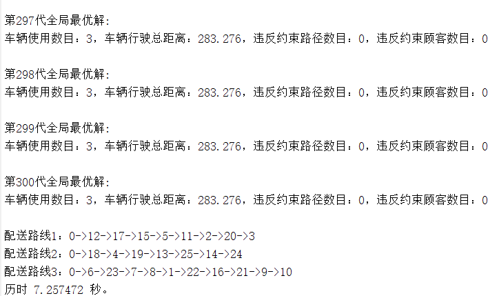
    %% Displays the distribution scheme information decoded by the current global optimal individual
    disp(['The first',num2str(gen),'Generation global optimal solution:'])
    [bestVC,bestNV,bestTD,best_vionum,best_viocus]=decode(bestInd,cusnum,cap,demands,dist);
    disp(['Number of vehicles used:',num2str(bestNV),'，Total vehicle distance:',num2str(bestTD),'，Number of constraint violation paths:',num2str(best_vionum),'，Number of customers violating constraints:',num2str(best_viocus)]);
    fprintf('\n')
    BestTD(gen,1)=bestTD;
    %% Update calculator
    gen=gen+1;
end
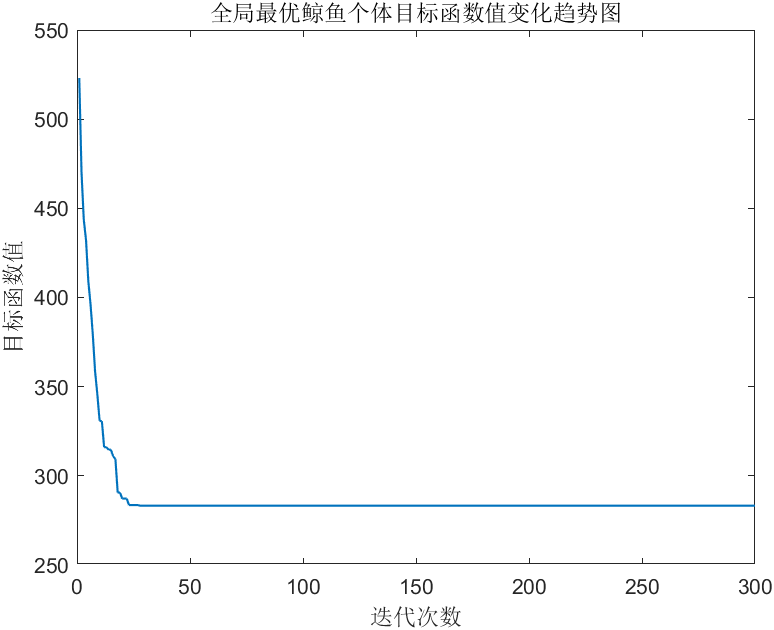
%% Print the total cost change trend of the global optimal solution of each iteration of the outer loop
figure;
plot(BestObj,'LineWidth',1);
title('Variation trend of individual objective function value of global optimal whale')
xlabel('Number of iterations');
ylabel('Objective function value');
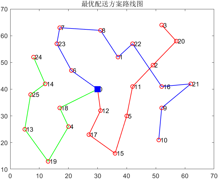
%% Print the global optimal solution roadmap. 1 means satisfied and 0 means dissatisfied
draw_Best(bestVC,vertexs);
toc