Moving target location algorithm

Detect the target in real time and locate the target in real time.

1. Computer simulation modeling of moving target

Assuming that the target moves in a uniform straight line and the position of the ith observation station is (x,y), the target motion model can be written as follows:

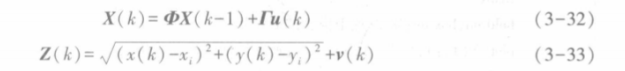
Of which:
Note: Γ \Gamma Γ G is used for simulation

The mean square deviation of u(k) Q=Wdiag([1,1]), W is an adjustable parameter, w < < 1. The mean square deviation of v(k) R=5

For example, in a 100mx 100m environment, use a computer to simulate the uniform motion of a target, as shown in formula (3-32). The target is affected by air resistance, resulting in different motion trajectories: it must be a uniform straight line, that is, the target has a certain trajectory jitter or bending. Assuming that the initial position of the target is (0,0) and the speed is (0.8,0.6), the process noise variance can be set to different sizes to observe the computer simulated target trajectory.

function TargetMotionModel %Computer simulation target motion model
dt=1;            %Sampling time,Company:second
Time=30;         %Total simulation time, also known as steps
X=zeros(4,Time); %Target in Time Status initialization at each time in time
x0=0;y0=0;vx=0.8;vy=0.6; %Target initial state, including position and speed
X(:,1)=[x0,vx,y0,vy]'; %The state of the first moment,Also called initial state
%System information, different systems,The state transition matrix and process noise driving matrix are also different
F=[1 dt 0 0;0 1 0 0;0 0 1 dt;0 0 0 1]; %formula(3-32)Mediumφ
G=[dt^2/2 0;dt 0;0 dt^2/2;0 dt]; %formula(3-32)Medium r
Q=0.1; %formula(3-32)in u(k)Variance of,Process noise
u=sqrt(Q)*randn(2,Time) ;
%Now start simulating the target over time,Start position movement
for k= 2:Time
    X(:,k)=F*X(:,k-1)+G*u(:,k);
end
figure
hold on;box on;%Set the display form of the coordinate axis
plot(X(1,:),X(3,:),'-r.');%Draw the trajectory of the target

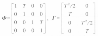
Operation results:

From left to right respectively, when Q=0.00001, the target basically moves in a straight line at a uniform speed; When Q=0.001, the trajectory of the target has begun to bend; When Q=0.1, it is impossible to believe that the target is moving in a uniform straight line, because the process noise is very large, resulting in the randomness of the target.

2. Moving target positioning based on distance observation

It is assumed that there are three or more observation stations to observe the target
The measurement equation of i observation stations is:

Finally, the distance information measured by these observation stations is transmitted to the fusion center, and the fusion center can realize the dynamic positioning of moving targets by using the least square method.

Example: in two-dimensional plane space, suppose the target moves in a uniform linear motion, the initial state of the target motion Is x(0)=[0,1.5,20,1.4], and the target has process noise under the influence of friction. In the environment, five observation stations detect the target distance. The measurement noise variance of the sensor in the observation station Is R=1, the sampling time Is, and the total running time Is 60s. The MATLAB simulation Is as follows:

function TrackingByDist %Distance based tracking(Continuous positioning)
%Basic information of the system model, including site size and location of observation stations.Model driven parameters, etc
Length=100;                          %Site space in meters
Width=100;                           %Site space in meters
Node_number=5;                       %Number of observation stations,There must be at least 3
for i=1:Node_number                  %Position initialization of observation station,The position here is given randomly
    Node(i).x= Width * rand;
    Node(i).y= Length * rand;
    Node(i).D= Node(i).x^2+Node(i).y^2; % Fixed parameters facilitate location estimation
end
T=1;                                 %Radar sampling time,Company:second
N= 60/T;                             %Total number of samples
delta_w=1e-3;                         %If you increase this parameter,The real trajectory of the target is a curve
Q=delta_w*diag([0.5,1]) ;             %Process noise mean
R=1;                                 %Observation noise variance
G=[T^2/2,0;T,0;0,T^2/2;0,T];         %Process noise driving matrix
F=[1,T,0,0;0,1,0,0;0,0,1,T;0,0,0,1]; %State transition matrix

%Start simulating target motion,Observations are sampled simultaneously in target motion,Measuring distance
X(:,1)=[0,1.5,20,1.4];               %Target initial position, speed, state parameter format[x,vx,y,vy]
Z=zeros( Node_number,N);            %Position observation by sensors at each observation station
Xn=zeros(2,N);                       %Least squares estimated position
for t=2:N                            %Modeling of equation of state:Target motion,Time from 1 T→NT
    X(:,t)=F*X(:,t-1)+G * sqrtm(Q) * randn(2,1); % Target real trajectory
end
for t=1:N                            %Modeling of observation equation:Multi station observation target, time from 1 T→NT
    for i= 1:Node_number             %Measurement of target distance at one time by one observation station
        [d1,d2]=DIST(X(:,t),Node(i)); %dl It's the real distance,d2 Is the square of the true distance
        Z(i,t)= d1+sqrtm(R) * randn; %The simulated observation distance is polluted by noise
    end
    %Double multiplication estimation of target position at current time
    A=[];b=[];
    for i=2:Node_number
        A(i-1,:)= 2*[Node(i).x-Node( 1).x,Node(i).y-Node(1).y];
        b(i-1,1)= [Z(1,t)^2-Z(i,t)^2+Node(i).D-Node(1).D];
    end
    Xn(:,t)= inv(A'*A)*A'*b;          %Get the current position of the target
end
for t=1:N                             %Calculate the position deviation, that is, use the least square position to make a difference with the real position of the target simulated by the computer
    error(t)=sqrt( (X(1,t)-Xn(1,t))^2+(X(3,t)-Xn(2,t))^2);
end
%Drawing
figure             %Trajectory diagram
hold on;box on;xlabel('x/m');ylabel('y/m');       %Frame for exporting drawings
for i= 1: Node_number
    h1= plot(Node(i).x, Node(i).y,'ko','MarkerFace','g','MarkerSize',10);
    text(Node(i).x+2,Node(i).y,[ 'Node ', num2str(i)]);
end
h2=plot(X(1,:),X(3,:),'-r'); %The real location of the target
h3=plot(Xn(1,:),Xn(2,:),'-k.'); %Estimated location of target
legend([h1,h2,h3 ],'Observation Station','Target Postion','Estimate Postion');
figure %Deviation diagram
hold on;box on;xlabel( 'time/s' );ylabel( 'value of the deviation');
plot( error,'-ko' ,'MarkerFace','g');

%Subfunction,Calculate the distance between two points and the square of the distance
function [dist ,dist2]=DIST(A,B)
dist2=(A(1)-B.x)^2+(A(3)-B.y)^2; %Square of distance
dist=sqrt(dist2); %distance
end

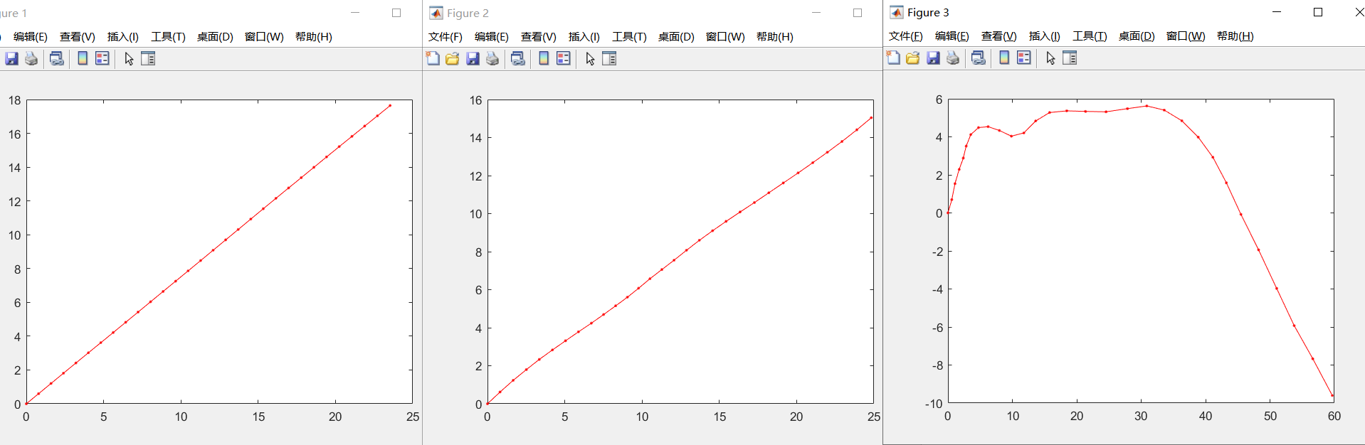
Operation results:

The figure shows the comparison between the positioning estimation and the real trajectory, and the figure on the right shows the comparison between the positioning estimation and the real position deviation.

Note: deviation is defined as

3. Azimuth only moving target positioning

Example: