In many scenarios, we need to decompose the signal to facilitate our next operation. The commonly used decomposition methods can include EMD family, such as EMD, EEMD, FEEMD, CEEMDAN, ICEEMDAN, etc. of course, there are also wavelet decomposition and empirical wavelet decomposition. In short, there are many decomposition methods. Different decomposition methods are selected according to the characteristics of samples. VMD decomposition is briefly introduced here.

Konstantin et al. Proposed a completely non recursive (VMD) in 2014, which can extract decomposition modes at the same time. The model looks for a set of modes and their respective center frequencies, so that these modes can reproduce the input signal together, and each mode is smooth after demodulation to the baseband. The essence of the algorithm is to extend the classical Wiener filter to multiple adaptive bands, which makes it have a solid theoretical foundation and easy to understand. The alternating direction multiplier method is used to effectively optimize the variational model, which makes the model more robust to sampling noise.

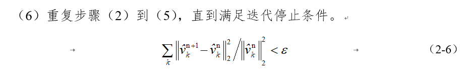
The specific process of VMD decomposition can be understood as the optimal solution of variational problem, and can be transformed into the construction and solution of variational problem.

 

 

The above is the theoretical part of VMD (variational modal decomposition). You may not understand it all, because I can't fully understand the mathematical relationship after reading the original text. Generally know which steps are involved in the decomposition process. There are many articles on this kind of decomposition on HowNet. You can refer to browse and learn.

Here's the code.

function [u, u_hat, omega] = VMD(signal, alpha, tau, K, DC, init, tol)
% Variational Mode Decomposition
% Authors: Konstantin Dragomiretskiy and Dominique Zosso
% zosso@math.ucla.edu --- http://www.math.ucla.edu/~zosso
% Initial release 2013-12-12 (c) 2013
%
% Input and Parameters:
% ---------------------
% signal  - the time domain signal (1D) to be decomposed
% alpha   - the balancing parameter of the data-fidelity constraint
% tau     - time-step of the dual ascent ( pick 0 for noise-slack )
% K       - the number of modes to be recovered
% DC      - true if the first mode is put and kept at DC (0-freq)
% init    - 0 = all omegas start at 0
%                    1 = all omegas start uniformly distributed
%                    2 = all omegas initialized randomly
% tol     - tolerance of convergence criterion; typically around 1e-6
%
% Output:
% -------
% u       - the collection of decomposed modes
% u_hat   - spectra of the modes
% omega   - estimated mode center-frequencies
%
% When using this code, please do cite our paper:
% -----------------------------------------------
% K. Dragomiretskiy, D. Zosso, Variational Mode Decomposition, IEEE Trans.
% on Signal Processing (in press)
% please check here for update reference: 
%          http://dx.doi.org/10.1109/TSP.2013.2288675


%---------- Preparations

% Period and sampling frequency of input signal
save_T = length(signal);
fs = 1/save_T;

% extend the signal by mirroring
T = save_T;
f_mirror(1:T/2) = signal(T/2:-1:1);
f_mirror(T/2+1:3*T/2) = signal;
f_mirror(3*T/2+1:2*T) = signal(T:-1:T/2+1);
f = f_mirror;

% Time Domain 0 to T (of mirrored signal)
T = length(f);
t = (1:T)/T;

% Spectral Domain discretization
freqs = t-0.5-1/T;

% Maximum number of iterations (if not converged yet, then it won't anyway)
N = 500;

% For future generalizations: individual alpha for each mode
Alpha = alpha*ones(1,K);

% Construct and center f_hat
f_hat = fftshift((fft(f)));
f_hat_plus = f_hat;
f_hat_plus(1:T/2) = 0;

% matrix keeping track of every iterant // could be discarded for mem
u_hat_plus = zeros(N, length(freqs), K);

% Initialization of omega_k
omega_plus = zeros(N, K);
switch init
    case 1
        for i = 1:K
            omega_plus(1,i) = (0.5/K)*(i-1);
        end
    case 2
        omega_plus(1,:) = sort(exp(log(fs) + (log(0.5)-log(fs))*rand(1,K)));
    otherwise
        omega_plus(1,:) = 0;
end

% if DC mode imposed, set its omega to 0
if DC
    omega_plus(1,1) = 0;
end

% start with empty dual variables
lambda_hat = zeros(N, length(freqs));

% other inits
uDiff = tol+eps; % update step
n = 1; % loop counter
sum_uk = 0; % accumulator



% ----------- Main loop for iterative updates




while ( uDiff > tol &&  n < N ) % not converged and below iterations limit
    
    % update first mode accumulator
    k = 1;
    sum_uk = u_hat_plus(n,:,K) + sum_uk - u_hat_plus(n,:,1);
    
    % update spectrum of first mode through Wiener filter of residuals
    u_hat_plus(n+1,:,k) = (f_hat_plus - sum_uk - lambda_hat(n,:)/2)./(1+Alpha(1,k)*(freqs - omega_plus(n,k)).^2);
    
    % update first omega if not held at 0
    if ~DC
        omega_plus(n+1,k) = (freqs(T/2+1:T)*(abs(u_hat_plus(n+1, T/2+1:T, k)).^2)')/sum(abs(u_hat_plus(n+1,T/2+1:T,k)).^2);
    end
    
    % update of any other mode
    for k=2:K
        
        % accumulator
        sum_uk = u_hat_plus(n+1,:,k-1) + sum_uk - u_hat_plus(n,:,k);
        
        % mode spectrum
        u_hat_plus(n+1,:,k) = (f_hat_plus - sum_uk - lambda_hat(n,:)/2)./(1+Alpha(1,k)*(freqs - omega_plus(n,k)).^2);
        
        % center frequencies
        omega_plus(n+1,k) = (freqs(T/2+1:T)*(abs(u_hat_plus(n+1, T/2+1:T, k)).^2)')/sum(abs(u_hat_plus(n+1,T/2+1:T,k)).^2);
        
    end
    
    % Dual ascent
    lambda_hat(n+1,:) = lambda_hat(n,:) + tau*(sum(u_hat_plus(n+1,:,:),3) - f_hat_plus);
    
    % loop counter
    n = n+1;
    
    % converged yet?
    uDiff = eps;
    for i=1:K
        uDiff = uDiff + 1/T*(u_hat_plus(n,:,i)-u_hat_plus(n-1,:,i))*conj((u_hat_plus(n,:,i)-u_hat_plus(n-1,:,i)))';
    end
    uDiff = abs(uDiff);
    
end


%------ Postprocessing and cleanup


% discard empty space if converged early
N = min(N,n);
omega = omega_plus(1:N,:);

% Signal reconstruction
u_hat = zeros(T, K);
u_hat((T/2+1):T,:) = squeeze(u_hat_plus(N,(T/2+1):T,:));
u_hat((T/2+1):-1:2,:) = squeeze(conj(u_hat_plus(N,(T/2+1):T,:)));
u_hat(1,:) = conj(u_hat(end,:));

u = zeros(K,length(t));

for k = 1:K
    u(k,:)=real(ifft(ifftshift(u_hat(:,k))));
end

% remove mirror part
u = u(:,T/4+1:3*T/4);

% recompute spectrum
clear u_hat;
for k = 1:K
    u_hat(:,k)=fftshift(fft(u(k,:)))';
end

end

The code is very long. Try to read as much as you can understand. I won't explain it here because it's a reproduction of mathematical principles. If you want to understand the principles, it's recommended to combine the original text with the code and read it line by line. If we only use this decomposition method to care about the results, there is no need to spend a lot of time.

function [u, u_hat, omega] = VMD(signal, alpha, tau, K, DC, init, tol)

Function input and output, here to explain.

The input part of the function: signal represents the input signal, alpha the first mock exam, the tau indicates the balance parameter of the data fidelity constraint, tau indicates the time step, K indicates the decomposition level, and DC indicates that if the first mode is placed in DC(0 frequency), then true. init represents the initialization of the signal and tol represents the convergence fault tolerance criterion. Generally, except K, that is, the number of decomposed modes, other parameters have corresponding empirical values. The exploration of VMD in most literature is also the determination of decomposition mode number, at most coupled with tau's discussion. (the blogger will also discuss it later.)

The output part of the function: u represents the set of decomposition modes, u_hat represents the spectral range of the mode, and omega represents the center frequency of the estimated mode.

The following is the main program to call VMD decomposition. The main step is to input the signal value, determine the decomposition parameters of VMD and draw the diagram.

tic
clc
clear all

load('IMF1_7.mat')
x=IMF1_7;
t=1:length(IMF1_7);


%--------- about VMD Set parameters---------------
alpha = 2000;       % moderate bandwidth constraint: Moderate bandwidth constraints/Penalty factor
tau = 0.0244;          % noise-tolerance (no strict fidelity enforcement): Noise tolerance (without strict fidelity)
K = 7;              % modes: Mode number of decomposition
DC = 0;             % no DC part imposed: No DC part
init = 1;           % initialize omegas uniformly  : omegas Uniform initialization of
tol = 1e-6 ;        
%--------------- Run actual VMD code:Data conduct vmd decompose---------------------------
[u, u_hat, omega] = VMD(x, alpha, tau, K, DC, init, tol);
figure;
imfn=u;
n=size(imfn,1); %size(X,1),Return matrix X Number of rows; size(X,2),Return matrix X Number of columns; N=size(X,2)，Is to put the matrix X The number of columns assigned to N




for n1=1:n
    subplot(n,1,n1);
    plot(t,u(n1,:));%output IMF weight, a(:,n)Then it represents the matrix a The first n Column elements, u(n1,:)Representation matrix u of n1 Row element
    ylabel(['IMF' ,int2str(n1)],'fontsize',11);%int2str(i)Yes, set the value i Rounded to characters, y Axis naming
end
 xlabel('Sample sequence','fontsize',14,'fontname','Song typeface');

%time\itt/s
 toc;
 

The following figure is recorded as the result of decomposition.

The above is a brief description of VMD decomposition. The following blog will discuss how to fix the decomposition layers accordingly.