
Taking the example of issue 16 as an example, we select Matlab and Excel to explain how to realize the general simplex method, large M method and two-stage method. The topics are as follows:

1, Matlab solution
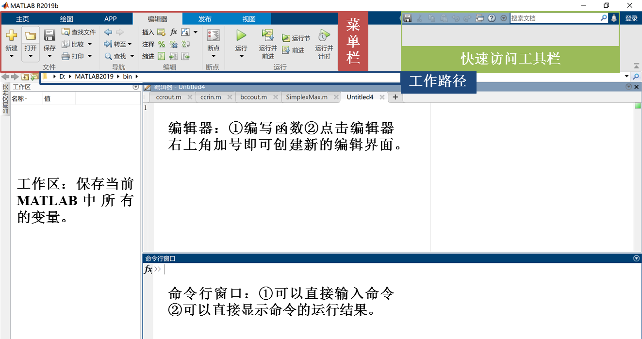
As one of the most popular scientific computing software, MATLAB is widely used in data analysis, wireless communication, deep learning, quantitative finance and risk management, control system and other fields. In order to make you better use the software, Xiaobian briefly introduces the MATLAB interface here: the interface is mainly composed of five functional areas: menu bar, quick access toolbar, workspace, editor and command line window. The functions of each area are as follows.
Algorithm implementation
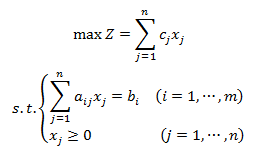
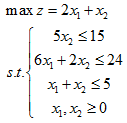
Before the example test using MATLAB platform, the linear programming problem needs to be transformed into a standard form:
As one of the mainstream tools for solving linear programming problems, matlab can find many relevant learning resources on the Internet. This time, based on the relevant resources shared by Mr. Zhang Jingxin of Harbin Business University on Zhihu platform, I will share with you the matlab code of simplex method and its expansion algorithm (big M method and two-stage method) and the specific implementation process of relevant examples.
First, write a general function for solving linear programming problems - SimplexMax in the MATLAB editor window
function [x,z,ST,res_case] = SimplexMax(c,A,b,ind_B)
% Input parameters: c Is the objective function coefficient, A Is the coefficient matrix of constraint equations, b Is the constant term of the constraint equations, ind_B Index the base variable;
%Output parameters: x Optimal solution, z Is the optimal objective function value, ST Storing simplex table data, res_case=0 Indicates that there is an optimal solution,
res_case=1 Indicates whether there is a bounded solution.
[m,n] = size(A);
%m Number of storage constraints
%n Number of decision variables stored
ind_N = setdiff(1:n, ind_B);
%Index of non base variable
ST = [];
format rat
% Use fractions to represent values
while true
% Circular solution
x0 = zeros(n,1);
x0(ind_B) = b;
%Initial basis feasible solution
cB = c(ind_B);
%calculation cB
Sigma = zeros(1,n);
Sigma(ind_N) = c(ind_N) - cB*A(:,ind_N);
%Calculate inspection number
[~, k] = max(Sigma);
%Select the maximum number of tests and determine the index of the base variable k
Theta = b ./ A(:,min(k));
%calculationθ
Theta(Theta<=0) = 10000;
q=find(Theta== min(Theta));
%Select the smallestθ
el = ind_B(max(q));
%Determine the base variable index el: There are multiple minimaθValue,
Select the variable with the largest subscript value.
vals = [cB',ind_B',b,A,Theta];
vals = [vals; NaN, NaN, NaN, Sigma, NaN];
ST = [ST; vals];
if ~any(Sigma > 0)
%The feasible solution is the optimal solution, any There is a>0
x = x0;
z = c * x;
res_case = 0;
return
end
if all(A(:,k) <= 0)
%Unbounded solution
x = [];
res_case = 1;
break
end
% Base replacement
ind_B(ind_B == el) = k;
%New base variable index
ind_N = setdiff(1:n, ind_B);
%Non base variable index
A(:,ind_N) = A(:,ind_B) \ A(:,ind_N);
b = A(:,ind_B) \ b;
A(:,ind_B) = eye(m,m);
% to update A and b
end
Second, input parameters in the command line window of MATLAB platform to complete the example solution
1. Simplex method

Test code:
A = [0 5 1 0 0;6 2 0 1 0;1 1 0 0 1];
% A Coefficient matrix of constraint equations
b = [15;24;5];
%b Is the constant term of constraint equations
c = [2 1 0 0 0];
% c Is the objective function coefficient
ind = [3 4 5];
%ind_d Index base variable
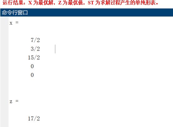
[x, z, ST, ca] = SimplexMax(c, A, b, ind)
%call SimplexMax function
%Click enter to output the results in the command line window.

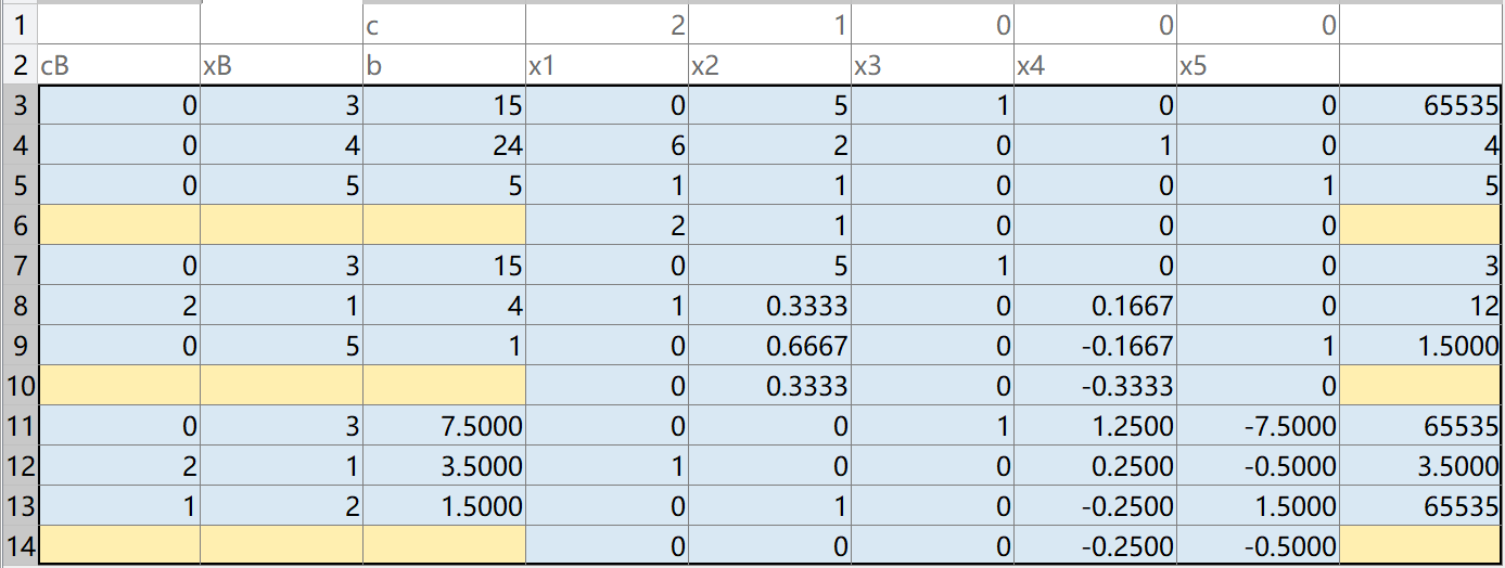
Write the running result to EXCEL:
xlswrite('SimplexTable1.xlsx', 'c', 1, 'C1');
% write in Excel
xlswrite('SimplexTable1.xlsx', {'cB','xB', 'b'}, 1, 'A2');
 [~,n] = size(A);
X = strcat('x', string(1:n));
% Write header
xlswrite('SimplexTable1.xlsx', X, 1, 'D2');
xlswrite('SimplexTable1.xlsx', c, 1, 'D1');
xlswrite('SimplexTable1.xlsx', ST, 1, 'A3');
% Write numerical results
2. Artificial variable method

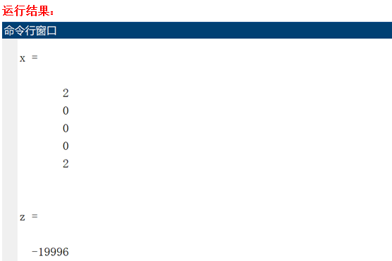
The implementation process of the large M method is almost the same as that of the simplex method. The only difference is that you need to set an infinite m value, and then call the SimplexMax function in the command line window to solve the problem.
Test code:
M=10000;
% assume M Infinity
A = [1 1 1 0 0;2 2 0 -1 1];
% A Coefficient matrix of constraint equations
b = [2;6];
% b Is the constant term of constraint equations
c = [2 1 0 0 -M];
% c Is the objective function coefficient
ind = [3 5];
%ind Index base variable
[x, z, ST, ca] = SimplexMax(c, A, b, ind)
%call SimplexMax function
%Click enter to output the results in the command line window.

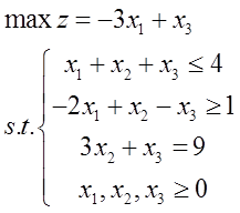
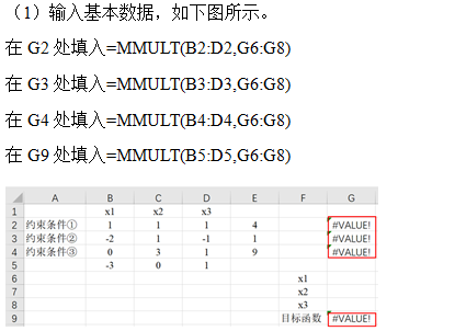
3. Two stage method
The two-stage method is to call SimplexMax twice, focusing on the connection between the two function calls.

Test code:
% Phase I
A1 = [1 1 1 1 0 0 0;-2 1 -1 0 -1 1 0; 0 3 1 0 0 0 1];
b1 = [4; 1; 9];
c1 = [0 0 0 0 0 -1 -1];
ind1 = [4 6 7];
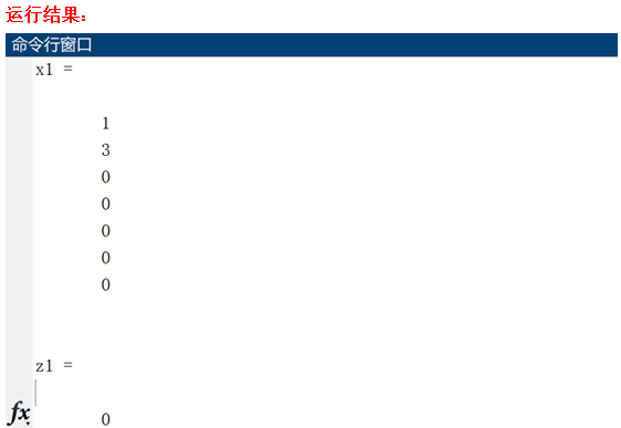
[x1, z1, ST1, ca1] = SimplexMax(c1, A1, b1, ind1)

% In the second stage, the artificial variables are removed
A2 = ST1(end-size(A1,1):end-1,4:end-3);   %2 Personal variables, 2+1
b2 = ST1(end-size(A1,1):end-1,3);
c2 = [-3 0 1 0 0];
ind2 = ST1(end-size(A1,1):end-1,2)';
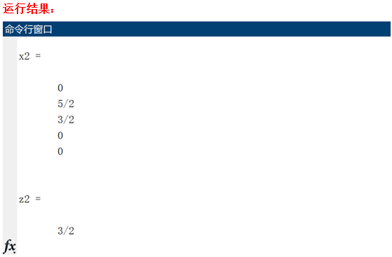
[x2, z2, ST2, ca2] = SimplexMax(c2, A2, b2, ind2)

2, Excel solution
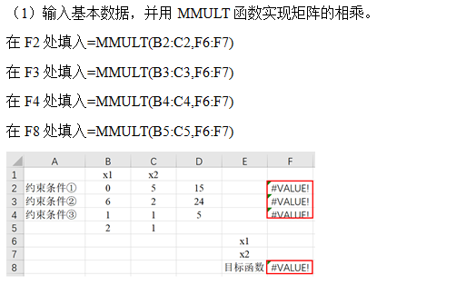
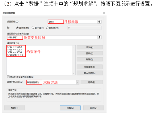
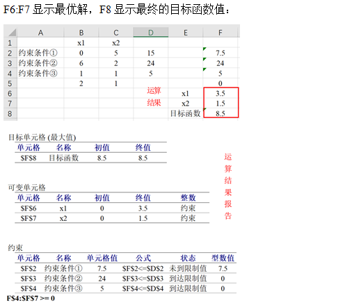
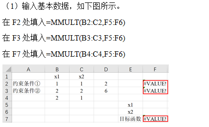
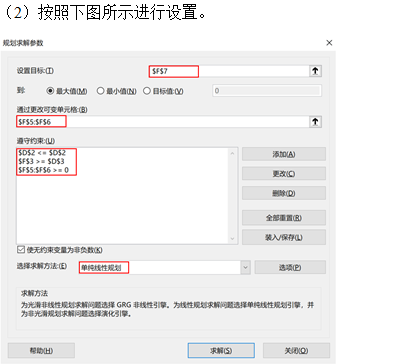
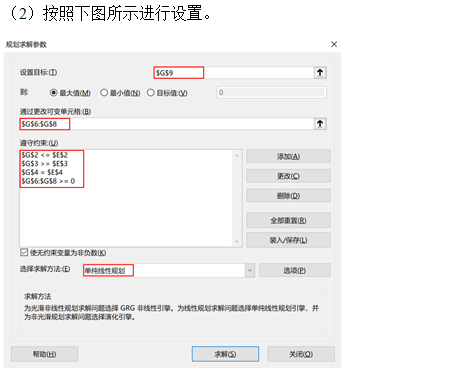
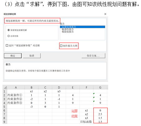
Before doing this, make sure that Excel is installed on our computer, and WPS table does not have this function! Then you need to install the solver module. The steps are "file - > Options - > add in - > go - > check the solver add in - > OK", so the "solver" item will appear in the "data" tab, and then we can use it.

1. Simplex method

2. Big M method
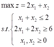
In EXCEL, the solving steps of artificial variable method and two-stage method are the same as that of simplex method.

3. Two stage method
Full text reference source:
https://zhuanlan.zhihu.com/p/61466360
https://zhuanlan.zhihu.com/p/61575249
https://blog.csdn.net/zsz_shsf/article/details/52837063
Author Chen Yimin, Cao Guiling
Editor in charge he Yangyang
Reviewed by Xu Xiaofeng
