1. The wolf species in the wolf swarm algorithm are divided into the following types:

Head wolf, probe wolf, fierce wolf.

2. Prey distribution rules: reward on merit, first strong and then weak.

3. The main body of the wolf swarm algorithm is composed of three intelligent behaviors: exploring wolf wandering, head wolf calling and fierce wolf siege, the "winner is the king" head wolf competition rule and the "survival of the fittest" wolf swarm update rule.

Step 1: randomly initialize the spatial coordinates of the wolves in the solution space, and drive out the artificial head wolf according to the size angle of the objective function value.

Step 2: the probe wolf starts to walk randomly and search for prey. If the objective function value of a certain position is found to be greater than the objective function value of the first wolf, the position of the first wolf will be updated, and the first wolf will send out calling behavior at the same time; If not found, the probe wolf continues to swim until the maximum number of walks is reached, and the head wolf sends out a call at the original position.

Step3: the fierce wolf who hears the call of the head wolf quickly rushes towards the head wolf in a large step. If the objective function value of the fierce wolf during the attack is greater than the objective function value of the head wolf, the position of the head wolf will be updated; Otherwise, the fierce wolf will continue to attack until it enters the siege range.

Step 4: the fierce wolf close to the head wolf will jointly detect the wolf to round up the prey (regard the position of the head wolf as the prey). During the round up process, if the objective function value of other artificial wolves is greater than the objective function value of the head wolf, the position of the head wolf will be updated until the prey is captured.

Step 5: eliminate the artificial wolves with small objective function value in the wolf pack, and randomly generate new artificial wolves in the solution space to realize the updating of the wolf pack.

Step 6: finally, judge whether the objective function value of the wolf meets the accuracy requirements or whether the algorithm reaches the maximum number of iterations.

4. Some rules of artificial wolf swarm algorithm:

(1) Rule of wolf generation

In the initial solution space, the artificial wolf with the optimal objective function value is the first wolf; In the process of iteration, the objective function value of the optimal wolf after each iteration is compared with the value of the first wolf in the previous generation. If it is better, the position of the first wolf is updated. If there are multiple wolves at this time, one is randomly selected as the first wolf. The first wolf does not perform three intelligent behaviors and directly enters the iteration until it is replaced by other stronger artificial wolves.

(2) Wandering behavior

The best s except the first Wolf_ Sum an artificial wolf is regarded as a probe wolf, S_sum random [n/ α+ 1，n/ α] Integer between, α Is the wolf scale factor.

Computational wolf detectionObjective function value of, ifGreater than the objective function value of the first Wolf, update the first wolf,=, detective WolfCall instead of the wolf; if>, then the probe wolf advances one step in h directions respectively (the swimming step is), record the function value after one step, then move forward in the direction p (p=1,2,...,h)The location is

                                                                       (1)

At this time, the function value of the location of the probe wolf is, select the function with the largest value and greater than the current function valueTake a step forward in the direction of and update the status of the probe wolf, repeat the above walking behavior until the function value of a probe wolf>Or the number of walks reaches the maximum number of walks.

Due to the different hunting methods of each probe wolf, thereforeThe values of are different, which can be taken in practiceRandom integers between,The larger the probe, the finer the search, but at the same time, the speed is relatively slow.

(3) Summoning behavior

Wolf callThe fierce wolf quickly drew close to the position of the first wolf； The fierce wolf takes a relatively large attack stepQuickly approach the wolf's position.

Fierce wolfNumberIn this iteration, the position is

                       (2)

Where,It is the position of the k-generation wolf. Equation (2) consists of two parts, the former is the current position of the artificial wolf, and the latter represents the trend that the artificial wolf gradually gathers to the position of the head wolf.

On the way, if a fierce wolfFunction value of, then, the fierce wolf transforms into a head wolf and initiates a summoning behavior; if, then the fierce wolfContinue to attack until it and the wolfDistance betweenless thanTurn into siege when.

Set the value range of the variable to be optimized as [lb,ub], then determine the distanceIt can be estimated by equation (3)

                                                                 (3)

Where,Is the distance determination factor,Increasing will accelerate the convergence of the algorithm, butThe over assembly makes it difficult for artificial wolves to enter the siege.

(4) Siege behavior

After the attack, the fierce wolf is close to the prey. At this time, the fierce wolf should jointly explore the wolf to siege and capture the prey. Here, the position of the wolf closest to the prey, that is, the head wolf, is regarded as the position where the prey moves. Specifically, for the k-generation wolf pack, the prey position is set as, the siege behavior of wolves can be expressed by equation (4):

                                     (4)

Where, is a random number evenly distributed among []; Attack step size when performing siege behavior for artificial wolf. If the concentration of prey odor perceived by the artificial wolf after the siege is greater than that perceived by its original position state, otherwise, the position of the artificial wolf remains unchanged.

5. Specific steps of artificial wolf swarm algorithm:

step1 value initialization;

Step 2 select the wolf and S_num an artificial wolf is a probe wolf and performs wandering behavior until a probe wolfThe odor concentration of prey detected at the bottom is greater than that perceived by the wolfOr reach the maximum number of walks, carry forward step3;

step3 the artificial fierce wolf attacks the prey according to equation (2), if the concentration of prey odor perceived by the fierce wolf on the way, then, instead of the first wolf to initiate summoning behavior; if, the artificial wolf continues to attack until, carry forward step4;

Step 4 updates the position of the artificial wolf participating in the siege according to formula (4) and executes the siege;

step5 update the position of the head wolf according to the rule of "the winner is the king"; Then the group renewal is carried out according to the wolf pack renewal mechanism of "survival of the strong";

Step 6 determines whether the optimization accuracy requirements or the maximum number of iterations are met. Otherwise, it is carried forward to step 2.

%% Empty environment
clc
clear all
close all
%% Data initialization

%Download data
load  HeightData
% HeightData=HeightData';
%Meshing
LevelGrid=10;
PortGrid=21;

%Start and end grid points
starty=6;starth=1;
endy=8;endh=21;
m=1;
%Algorithm parameters
PopNumber=10;         %Population number
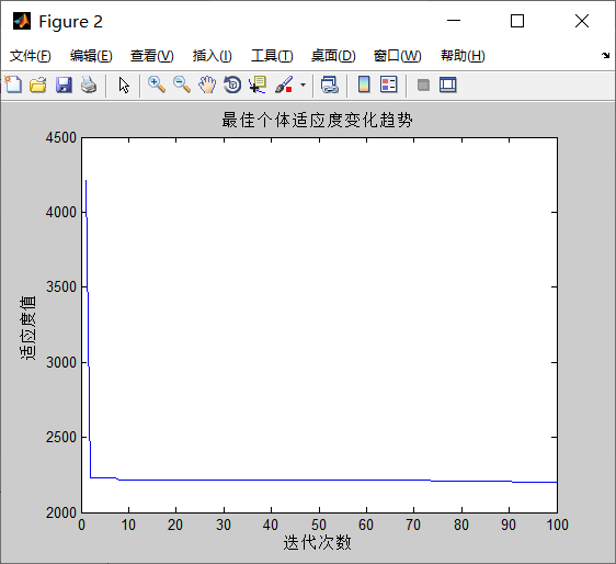
BestFitness=[];    %Best individual
iter=100;
%Initial pheromone
pheromone=ones(21,21,21);
dim=PortGrid*2;
Max_iter=100;
ub=PortGrid;
lb=1;
% initialize alpha, beta, and delta_pos
Alpha_pos=zeros(1,dim);
Alpha_score=inf; %change this to -inf for maximization problems
Beta_pos=zeros(1,dim);
Beta_score=inf; %change this to -inf for maximization problems
Delta_pos=zeros(1,dim);
Delta_score=inf; %change this to -inf for maximization problems
%Initialize the path of search agents
Convergence_curve=zeros(1,Max_iter);
l=0;% Loop counter
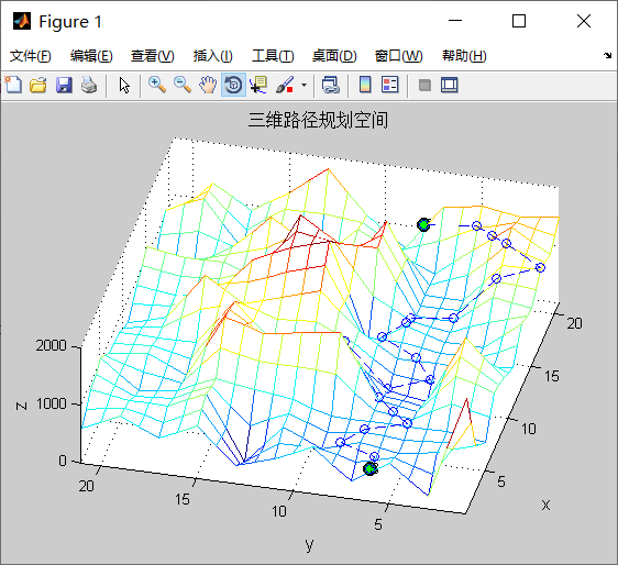
%% Initial search path
[path,pheromone]=searchpath(PopNumber,LevelGrid,PortGrid,pheromone, ...
    HeightData,starty,starth,endy,endh);
fitness=CacuFit(path);                          %Fitness calculation
[bestfitness,bestindex]=min(fitness);           %Optimum fitness
bestpath=path(bestindex,:);                     %Best path
BestFitness=[BestFitness;bestfitness];          %Fitness value record

l=0;% Loop counter

% Main loop
while l<Max_iter
    for i=1:size(path,1)
        
        % Return back the search agents that go beyond the boundaries of the search space
        Flag4ub=path(i,:)>ub;
        Flag4lb=path(i,:)<lb;
        path(i,:)=round((path(i,:).*(~(Flag4ub+Flag4lb)))+ub.*Flag4ub+lb.*Flag4lb);
        
        % Calculate objective function for each search agent
        fitness=CacuFit(path(i,:));
        
        % Update Alpha, Beta, and Delta
        if fitness<Alpha_score
            Alpha_score=fitness; % Update alpha
            Alpha_pos=path(i,:);
        end
        
        if fitness>Alpha_score && fitness<Beta_score
            Beta_score=fitness; % Update beta
            Beta_pos=path(i,:);
        end
        
end