fuzzy mathematics
What is fuzzy mathematics?
Fuzzy mathematics, also known as fuzzy mathematics or fuzzy mathematics. After 1965, fuzzy topology, fuzzy measure theory and other mathematical fields developed on the basis of fuzzy set and fuzzy logic. It is a mathematical tool to study many unclear or even fuzzy problems in the real world. It is widely used in pattern recognition, artificial intelligence and so on.
Next, we mainly introduce fuzzy sets and fuzzy comprehensive evaluation.
Fuzzy set
Many phenomena and relationships in reality are vague. Such as high and low, long and short, large and small, more and less, poor and rich, good and bad, young and old, etc.
This kind of phenomenon does not satisfy the exclusionary law of "either this or that", but has the fuzziness of "either this or that".
It should be pointed out that fuzzy uncertainty is different from random uncertainty. Random uncertainty is the uncertainty caused by the breakage of causality law, while fuzzy uncertainty is the uncertainty caused by the breakage of exclusion law.
In order to study fuzzy phenomena and relations, American cybernetics expert ZAD introduced the concept of fuzzy set in 1965.
Definition and representation
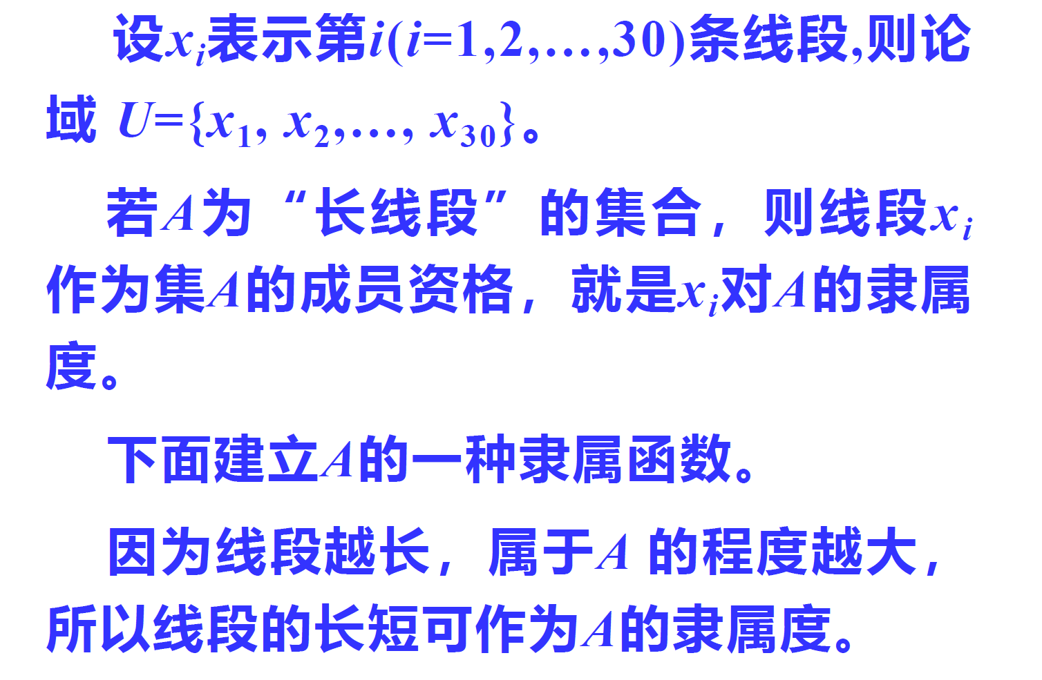
Given a universe U U U. So called U U Fuzzy sets on U A A A means for any x ∈ A x \in A x ∈ A can determine A positive number μ A ( x ) ∈ [ 0 , 1 ] \mu_A(x) \in [0,1] μ A (x) ∈ [0,1], expressed by x x x belongs to A A The degree of A.
mapping x ∈ U → μ A ( x ) ∈ [ 0 , 1 ] x \in U \rightarrow \mu_{A}(x) \in[0,1] x∈U→ μ A (x) ∈ [0,1] is called A A Membership function of A.
function μ A ( x ) \mu_A(x) μ A (x) is called x x x-pair fuzzy set A A Membership of A.
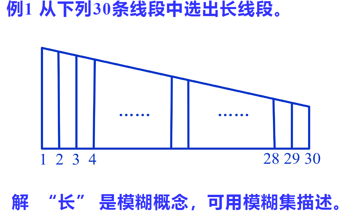
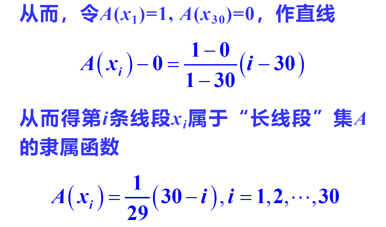
An example is given to illustrate how to construct membership
Operation of fuzzy sets
Because there is no absolute membership relationship between elements and sets in fuzzy set, the operation of fuzzy set is completed by membership function.
Let the membership functions of fuzzy sets a and B be
μ
A
(
x
)
\mu_A(x)
μA(x),
μ
B
(
x
)
\mu_B(x)
μ B (x), then the common operations of A and B are
KaTeX parse error: Undefined control sequence: \hfill at position 65: …\leq \mu_{B}(x)\ ̲ h ̲ f ̲ i ̲ l ̲ l ̲ ̲\ (2) Equal: A=B
Determination of membership function
According to the concept of fuzzy set, the basic idea of fuzzy mathematics is membership degree, so the key to establish mathematical model by using fuzzy mathematics method is to establish practical membership function.
However, how to determine the membership function of a fuzzy set is still an unsolved problem.
The common method to determine the membership degree is the fuzzy distribution method. The fuzzy distribution method regards the membership function as a fuzzy distribution. Firstly, the appropriate fuzzy distribution is selected according to the nature of the problem, and then the parameters in the distribution are determined according to the relevant data.
The trapezoidal distribution commonly used in fuzzy distribution is briefly introduced below.
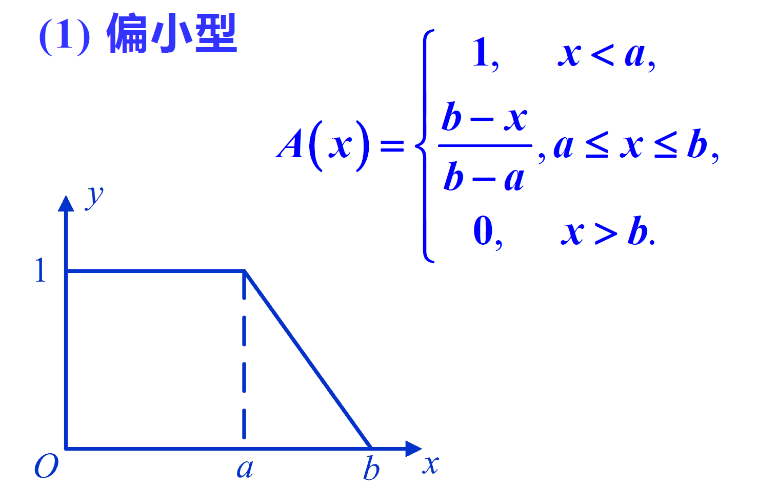
Small
Larger
Intermediate type
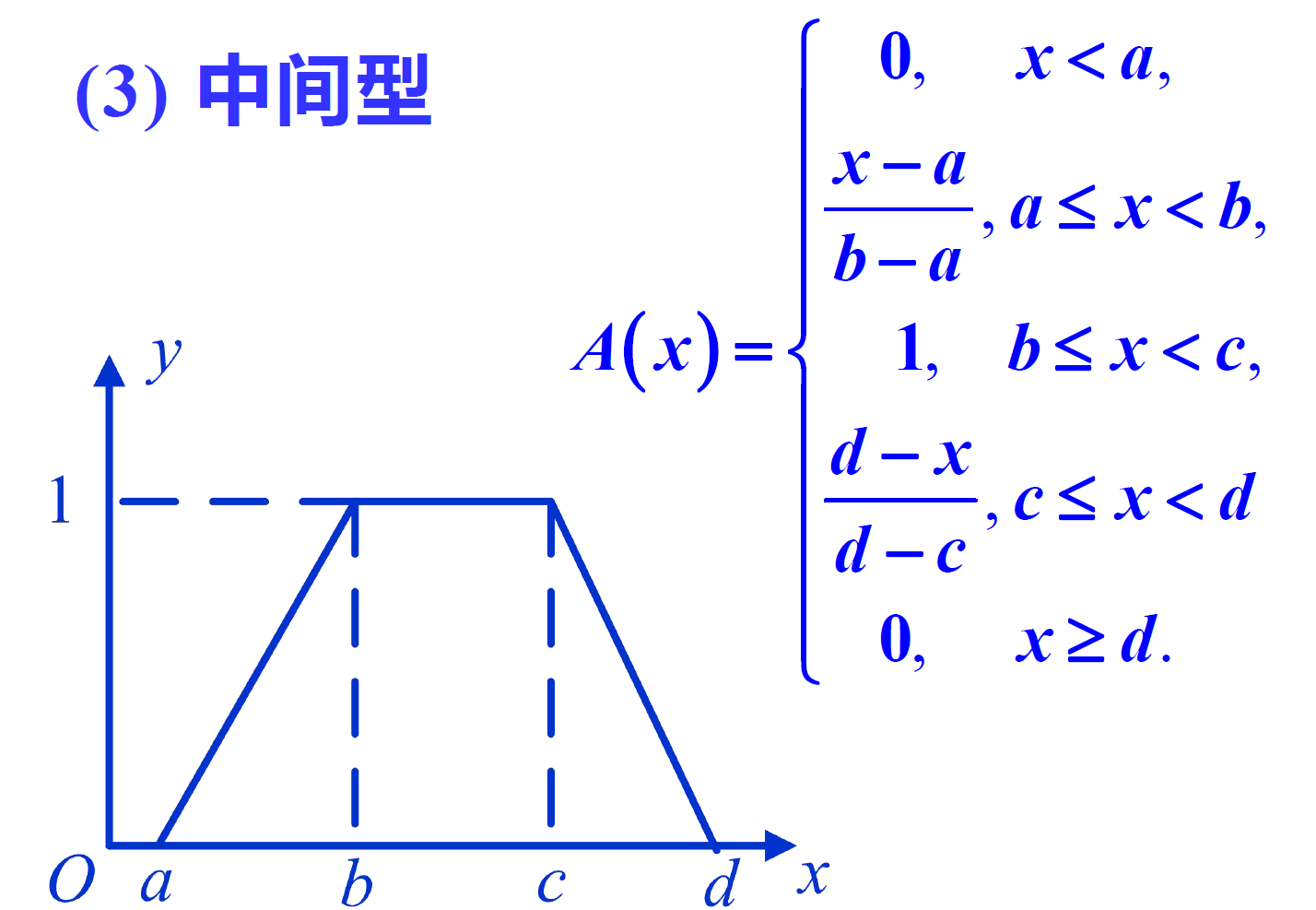
Small is generally suitable for describing fuzzy phenomena with small degree, such as "small", "little", "shallow" and "light"; Relatively large is just the opposite of relatively small; The intermediate type is generally suitable for describing the fuzzy phenomenon in the intermediate state.
Fuzzy comprehensive evaluation
Evaluation is a regular and extremely important cognitive activity in human society.
The evaluation of a thing usually involves multiple factors or indicators. Evaluation is a comprehensive evaluation under the interaction of multiple factors.
Comprehensive evaluation is a common problem in mathematical modeling competition, such as:
- Evaluation and prediction of water quality in the Yangtze River (2005A)
- Evaluation of AIDS therapy and prediction of curative effect (2006B)
- Quantitative evaluation of the influence of 2010 Shanghai World Expo (2010B).
There are many comprehensive evaluation methods, such as grey evaluation method, analytic hierarchy process, fuzzy comprehensive evaluation method, data envelopment analysis method, artificial neural network evaluation method, ideal solution and so on. Sometimes, the two evaluation methods can be integrated into a combined evaluation method.
Various evaluation methods have different starting points, different ideas to solve problems, different applicable objects, and have their own advantages and disadvantages. Different evaluation methods will produce different evaluation conclusions, sometimes even different conclusions, that is, the result of comprehensive evaluation is not unique.
As a specific application of fuzzy mathematics, fuzzy comprehensive evaluation was first proposed by Chinese scholar Wang peizhuang. The basic idea is: Based on fuzzy mathematics and the principle of fuzzy relationship synthesis, quantify some factors with unclear boundary and difficult to quantify, and comprehensively evaluate the subordinate level of the evaluated things from multiple factors.
The specific steps are as follows: firstly, determine the factor set and evaluation set of the evaluated object, then determine the weight of each factor and their membership vector respectively, and obtain the fuzzy evaluation matrix. Finally, the fuzzy evaluation matrix and the factor weight vector are fuzzy calculated and normalized, so as to obtain the comprehensive result of fuzzy evaluation.
The fuzzy comprehensive evaluation method is simple and easy to master. It has a good evaluation effect on multi factor and multi-level complex problems, and is difficult to be replaced by other evaluation methods.
1. Determine the evaluation index and evaluation level
set up U = u 1 , u 2 , . . . , u m U={u_1,u_2,...,u_m} U=u1,u2,..., um ^ is the description of the evaluated object m m m) three factors, namely evaluation index;
V = v 1 , v 2 , . . . , v n V={v_1,v_2,...,v_n} V=v1,v2,..., vn ^ is the description of the state of each factor n n n kinds of comments, namely evaluation grade.
here, m m m is the number of evaluation factors, which is usually determined by the specific index system; n n n is the number of comments, generally divided into 3 ~ 5 levels.
For example, a garment factory wants to use the fuzzy comprehensive evaluation method to understand the customer's welcome to a certain garment.
Whether customers like a certain garment is usually related to the design, style, price, durability and comfort of the garment, so the factor set for evaluating the garment is determined as
U
=
{
flower
colour
,
kind
type
,
price
grid
,
Endure
use
degree
,
Comfortable
suitable
degree
}
U=\left \ {decor, style, price, durability, comfort \ right \}
U = {decor, style, price, durability, comfort}
The purpose of comprehensive evaluation is to find out the customer's welcome to all aspects of clothes. Therefore, the evaluation set should be
V
=
{
very
Joyous
Welcome
,
Joyous
Welcome
,
one
like
,
no
Joyous
Welcome
}
V=\left \ {very welcome, welcome, general, not welcome \ right \}
V = {very welcome, welcome, general, not welcome}
2. Construct fuzzy comprehensive evaluation matrix
After determining the evaluation index and evaluation grade, it is necessary to evaluate each evaluation index u i ( i = 1 , 2 , ... m ) {u}_{i}(i=1,2, \ldots {m}) ui (i=1,2,... m) was evaluated one by one.
The specific evaluation method is: the evaluation index u i u_i ui) give a rating that it can be rated v i v_i vi. membership of r i j r_{ij} rij.
r i j r_{ij} rij# can be understood as an indicator u i u_i ui # for Grades v i v_i vi , membership, usually r i j r_{ij} rij# normalized for ease of use.
Let the fuzzy evaluation of the index ${u}{i} $be ${r} {I} = \ left ({r} {I 1}, {r} {I 2} \ right,, \ left. \ ldots, R {i n} \ right) $, then all evaluation indexes $U_ {i} (I = 1,2, \ ldots, m) $
R
=
(
r
i
j
)
m
×
n
=
(
r
11
r
12
⋯
r
1
n
r
21
r
22
⋯
r
2
n
⋮
⋮
⋱
⋮
r
m
1
r
m
2
⋯
r
m
n
)
{R}=\left({r}_{i j}\right)_{m \times n}=\left(\begin{array}{cccc} {r}_{11} & {r}_{12} & \cdots & {r}_{1 n} \\ {r}_{21} & {r}_{22} & \cdots & {r}_{2 n} \\ \vdots & \vdots & \ddots & \vdots \\ {r}_{m 1} & {r}_{m 2} & \cdots & {r}_{m n} \end{array}\right)
R=(rij)m×n=⎝⎜⎜⎜⎛r11r21⋮rm1r12r22⋮rm2⋯⋯⋱⋯r1nr2n⋮rmn⎠⎟⎟⎟⎞
It is called the fuzzy comprehensive evaluation matrix of each index.
The frequency method is usually used to determine the membership degree r i j r_{ij} rij. For example, in the previous example, for the design and color of the clothing, 20% of the respondents think it is "very welcome", 50% think it is "welcome", 30% think it is "average", and no one thinks it is "not welcome", then the evaluation vector of u1 is R 1 = ( 0.2 , 0.5 , 0.3 , 0 ) R_1=(0.2,0.5,0.3,0) R1=(0.2,0.5,0.3,0).
Similarly, the evaluation vector of other indicators is
KaTeX parse error: Undefined control sequence: \hfill at position 25: ...(0.2,0.5,0.3,0)\̲h̲f̲i̲l̲l̲ ̲\\R_{2} = (0.1,...
Thus, the fuzzy comprehensive evaluation matrix is
A
=
(
0.2
0.5
0.3
0
0.1
0.3
0.5
0.1
0
0.1
0.6
0.3
0
0.4
0.5
0.1
0.5
0.3
0.2
0
)
A=\left(\begin{array}{cccc} 0.2 & 0.5 & 0.3 & 0 \\ 0.1 & 0.3 & 0.5 & 0.1 \\ 0 & 0.1 & 0.6 & 0.3 \\ 0 & 0.4 & 0.5 & 0.1 \\ 0.5 & 0.3 & 0.2 & 0 \end{array}\right)
A=⎝⎜⎜⎜⎜⎛0.20.1000.50.50.30.10.40.30.30.50.60.50.200.10.30.10⎠⎟⎟⎟⎟⎞
3. Determination of evaluation index weight
The fuzzy comprehensive evaluation matrix is determined, which is not enough to evaluate things. The reason is that each evaluation index has different positions and functions in the evaluation objectives, that is, each evaluation index occupies different weights in the comprehensive evaluation.
A fuzzy vector is usually introduced A = ( a 1 , a 2 , ... , a n ) A=(a_1,a_2,...,a_n) A=(a1, a2,..., an) represents the weight of each evaluation index in the target, which is called the weight vector.
Of which $a_{i} $is the weight of ${u}{i} $, $a{i} \geq 0, \sum a_{i}=1$
There are usually subjective and objective methods to determine the weight.
The representative of subjective method is analytic hierarchy process.
The objective method uses mathematical methods to calculate the weight of each index according to the relationship between each index, such as mass fraction method, coefficient of variation method, etc. The coefficient of variation method is introduced with examples.
Coefficient of variation method
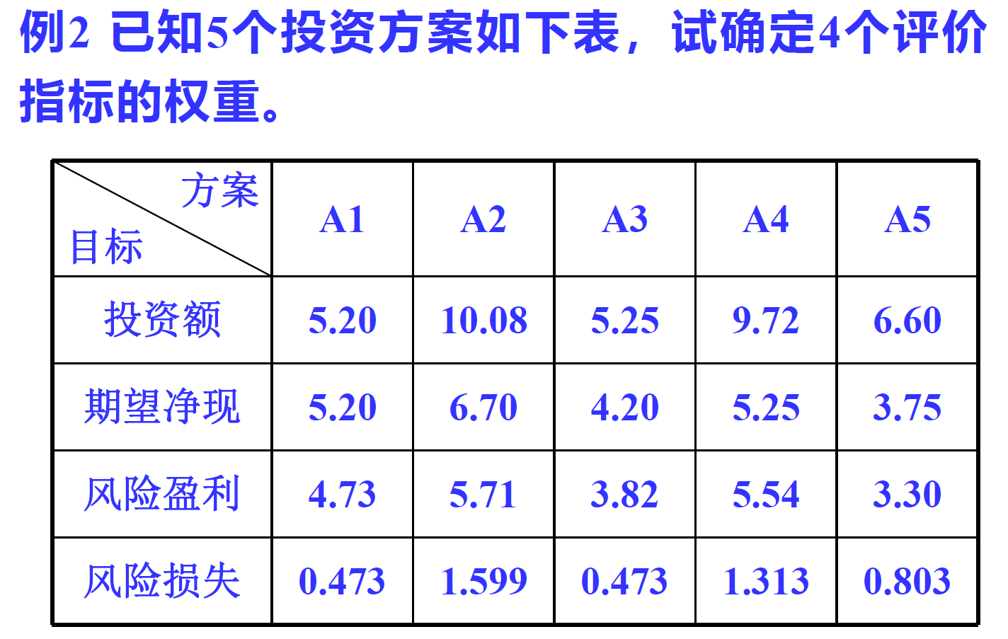
The design principle of the coefficient of variation method is: if the value of an index is greatly different, it can clearly distinguish the evaluated objects, indicating that the index has rich resolution information, so a large weight should be given to the index; On the contrary, if the value difference of each evaluated object in an index is small, the ability of this index to distinguish each evaluated object is weak, so the index should be given a small weight.
Because variance can describe the dispersion of values, that is, the variance of an index reflects the resolution of the index, the weight of the index can be defined by variance.
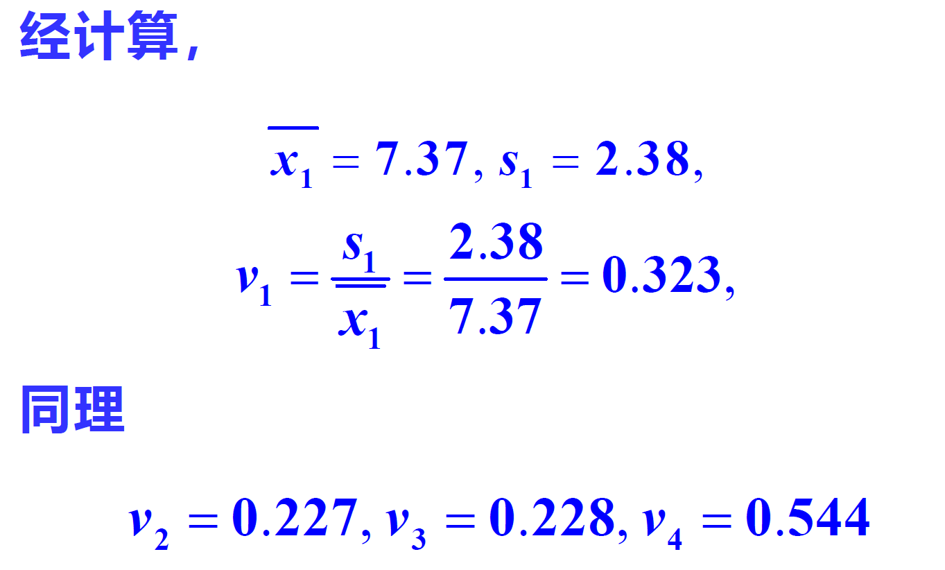
Since the magnitude of variance is relative and the magnitude and magnitude of the index value need to be considered, the resolution of the index can be defined as
v
i
=
s
i
/
∣
x
ˉ
i
∣
v_{i}=s_{i} /\left|\bar{x}_{i}\right|
vi=si/∣xˉi∣
Code implementation of coefficient of variation method
a = [5.20 10.08 5.25 9.72 6.60;
5.20 6.70 4.20 5.25 3.75;
4.73 5.71 3.82 5.54 3.30;
0.473 1.599 0.473 1.313 0.803];

wi = var_coefficient(a)

%% The weight of each index is calculated by coefficient of variation method
function y=var_coefficient(a)
    [m,n] = size(a);
    si2 = zeros(1, m);
    % m Two indicators, n Kinds of schemes
    for i=1:m
        % The first i Mean value of indicators
        mean_xi(i) = sum(a(i, :))/n;
        for j=1:n
            % The first i Variance of indicators
            si2(i) = si2(i)+(a(i, j)-mean_xi(i)).^2;
        end
        si2(i) = si2(i)/(n-1);
        si(i) = sqrt(si2(i));
        vi(i) = si(i)/abs(mean_xi(i));
    end
    for i=1:m
        wi(i) = vi(i)/sum(vi);
    end
    y = wi;
end
!! It should be pointed out that the weight of an index calculated by the coefficient of variation method and the importance of the index in the evaluation system are two concepts.
The function of coefficient of variation method is only to improve the resolution of indicators and facilitate sorting.
In fact, the premise of using the coefficient of variation method is that all indicators are of equal importance in the evaluation system.
In other words, when the importance of indicators in the evaluation system varies greatly, it is not necessarily appropriate to use the coefficient of variation method to determine the weight.
4. Fuzzy synthesis and comprehensive evaluation
Fuzzy comprehensive evaluation matrix R R Different lines in R reflect the subordinate degree of the evaluated object to each level from different index evaluation. Using weight vector A A A by synthesizing different rows, we can get the membership degree of the evaluated object to each level as a whole, that is, the fuzzy comprehensive evaluation result.
It is usually realized by so-called "fuzzy synthesis"
The basic idea of the above synthesis is: the evaluation matrix R R R and weight vector A A A performs some appropriate fuzzy operation to synthesize the two into a fuzzy vector B = ( b 1 , b 2 , ... , b n ) B=(b_1,b_2,...,b_n) B=(b1, b2,..., bn), i.e B = A R B=AR B=AR, then B B B the final fuzzy comprehensive evaluation result can be obtained after comprehensive analysis according to certain rules.
Common fuzzy composition operators are:
The characteristics of the above fuzzy synthesis operator are:
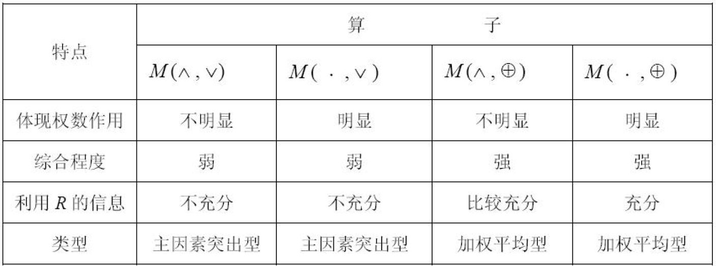
In fact, you can also take M M M is the ordinary matrix multiplication, and the synthesis is the weighted average. As for which operator to choose, it depends on the nature of the problem and the characteristics of the operator.
Generally, the results of using the main factor prominent algorithm and the weighted average algorithm are similar. But in practice, we should pay attention to the characteristics of these two kinds of algorithms.
The main factor prominent type is suitable for the situation where the data in the fuzzy matrix are very different, while the weighted average type is often used for the situation with many factors, which can avoid the loss of information.
Code implementation of synthesis operator
%% Composition operator M(^,v),input a Is the weight vector,r Fuzzy evaluation matrix
% The main factor prominent type is suitable for the situation that the data in the fuzzy matrix are widely different, and the weight effect is not obvious
function y=synthetic_arithmetic_1(a,r)
    [m,n] = size(r);
    for j=1:n
       for i=1:m
           h(i)=min([a(i),r(i,j)]);
       end
       b(j)=max(h);
    end
    %Normalization processing
    sum_b = sum(b);
    b = b./sum_b;
    y=b;
end

%% Composition operator M(.,v),input a Is the weight vector,r Fuzzy evaluation matrix
% The main factor prominent type is suitable for the situation that the data in the fuzzy matrix is widely different, and the weight function is obvious
function y=synthetic_arithmetic_2(a,r)
    [m,n] = size(r);
    for j=1:n
       for i=1:m
           h(i)=min([a(i)*r(i,j)]);
       end
       b(j)=max(h);
    end
    %Normalization processing
    sum_b = sum(b);
    b = b./sum_b;
    y=b;
end

%% Composition operator M(^,+),input a Is the weight vector,r Fuzzy evaluation matrix
% The weighted average type is suitable for the situation that the data in the fuzzy matrix are widely different, and the weight function is not obvious
function y=synthetic_arithmetic_3(a,r)
    [m,n] = size(r);
    b = zeros(1,n);
    for j=1:n
        tmp=0;
       for i=1:m
           tmp=tmp+min([a(i),r(i,j)]);
       end
       b(j)=tmp;
    end
    %Normalization processing
    sum_b = sum(b);
    b = b./sum_b;
    y=b;
end

%% Composition operator M(.,+),input a Is the weight vector,r Fuzzy evaluation matrix
% Weighted average type, which is suitable for the situation of wide difference in data in fuzzy matrix, and reflects the obvious role of weight
function y=synthetic_arithmetic_4(a,r)
    [m,n] = size(r);
    b = zeros(1,n);
    for j=1:n
        tmp=0;
       for i=1:m
           tmp=tmp+(a(i)*r(i,j));
       end
       b(j)=tmp;
    end
    %Normalization processing
    sum_b = sum(b);
    b = b./sum_b;
    y=b;
end
%% Calculate four composition operators, input a Is the weight vector,r Fuzzy evaluation matrix
function y=synthetic_arithmetic_all(a,r)
    y=[
        synthetic_arithmetic_1(a, r);
        synthetic_arithmetic_2(a, r);
        synthetic_arithmetic_3(a, r);
        synthetic_arithmetic_4(a, r)
];
end
B is called fuzzy comprehensive evaluation vector, b j b_j bj , meet $0 < B_ j <1 , And need want return one turn . , and normalization is required. , and normalization is required. b_j can reason solution by cover review price yes as yes The first It can be understood that the evaluated object It can be understood as the subordinate degree of the evaluated object to the j $level.
The comprehensive evaluation results can be obtained after analyzing and processing B. Common methods for analyzing and processing B include:
- The maximum membership method is to identify the grade of the evaluated object as the grade corresponding to the maximum membership. It is applicable to the situation that a certain membership degree is significantly greater than other membership degrees.
- Weighted average method: assign appropriate scores to each grade in the evaluation set $\ mathrm{V}=\left{\mathrm{v}{1}, \mathrm{v}{2}, \ldots, \mathrm{v}{\mathrm{n}}\right} $\ mathrm C=\left{c{1}, c_{2}, \ldots, c_{n}\right} $, using normalized comprehensive evaluation vector $\ mathrm{B}=\left{\mathrm{b}{1}, \mathrm{~b}{2}, \ldots, \mathrm{b}_{\mathrm{n}}\right} $weighted average of $\ mathrm{C} $
∑ i = 1 n c i b i \sum_{i=1}^{n} c_{i} b_{i} i=1∑ncibi
As the result of fuzzy comprehensive evaluation.
Example code implementation
%% Test
r = [0.4 0.5 0.1 0;
0.6 0.3 0.1 0;
0.1 0.2 0.6 0.1;
0.1 0.2 0.5 0.2];

a = [0.5,0.2,0.2,0.1];

B = [synthetic_arithmetic_1(a, r);
synthetic_arithmetic_2(a, r);
synthetic_arithmetic_3(a, r);
synthetic_arithmetic_4(a, r)
]

%% Or write it directly
B = synthetic_arithmetic_all(a, r)
% Output results
B =

    0.3333    0.4167    0.1667    0.0833
    0.3390    0.4237    0.2034    0.0339
    0.3200    0.4000    0.2000    0.0800
    0.3500    0.3700    0.2400    0.0400
5. Relative deviation fuzzy matrix evaluation method
The relative deviation fuzzy matrix evaluation method is somewhat similar to the grey correlation analysis. First, an ideal solution is proposed u u u. Then establish each scheme and model according to some method u u Deviation matrix of u R R R. Then determine the weight of each evaluation index A A A. Last use A A A yes R R R weighted average of each scheme and u u Comprehensive distance of u F F F. Then according to F F F to sort the schemes.
Relative deviation fuzzy matrix MATLAB general code implementation
%% Relative deviation fuzzy matrix,A Is the initial matrix,Each row represents each scheme and each column represents an indicator,good Number of columns representing benefit type
function y=rela_eviation_fuzzy(A,good)
    [m,n]=size(A);%Find out how many rows and columns
    maxA=max(A);%Find the maximum value of each column
    minA=min(A);%Find the minimum value of each column
    G=maxA-minA;%Maximum minus minimum
    u=[];
    for i1=1:n
        if contain(i1,good)==1
            u=[u,max(A(:,i1))];
        else
            u=[u,min(A(:,i1))];
        end
    end
    R=zeros(m,n);%Set the initial value of fuzzy synthesis matrix to 0
    % The fuzzy synthesis matrix is obtained as follows
    for i2=1:m
        for j=1:n
            R(i2,j)=abs(A(i2,j)-u(j))/G(j);
        end
    end
    y=R;

    function ab=contain(ele,vec)
        len=length(vec);
        res=0;
        for i=1:len
            if vec(i)==ele
                res=1;
            end
        end
        ab=res;
    end
end
Calculate the problem
%% Test relative deviation fuzzy matrix function rela_eviation_fuzzy(A,good)
clc;clear;
A=[1000 120 5000 1 50 1.5 1;
    700 60 4000 2 40 2 2;
    900 60 7000 1 70 1 4;
    800 70 8000 1.5 40 0.5 6;
    800 80 4000 2 30 2 5];
good=[1,7];
disp('--------------Deviation fuzzy matrix--------------')
r=rela_eviation_fuzzy(A,good)
disp('--------------According to the coefficient of variation method, the weight of each index is calculated as--------------')
wi = var_coefficient(A')
disp('-----------------Weighted mean variance of each scheme-------------------')
B=wi*r'
Calculation results
--------------Deviation fuzzy matrix--------------

r =

         0    1.0000    0.2500         0    0.5000    0.6667    1.0000
    1.0000         0         0    1.0000    0.2500    1.0000    0.8000
    0.3333         0    0.7500         0    1.0000    0.3333    0.4000
    0.6667    0.1667    1.0000    0.5000    0.2500         0         0
    0.6667    0.3333         0    1.0000         0    1.0000    0.2000

--------------According to the coefficient of variation method, the weight of each index is calculated as--------------

mean_xi =

   1.0e+03 *

    0.8400    0.0780    5.6000    0.0015    0.0460    0.0014    0.0036

Average value of each indicator:

mean_xi =

   1.0e+03 *

    0.8400    0.0780    5.6000    0.0015    0.0460    0.0014    0.0036

Standard deviation of each indicator:

si =

   1.0e+03 *

    0.1140    0.0249    1.8166    0.0005    0.0152    0.0007    0.0021

Weight of each indicator (no normalization)

vi =

    0.1357    0.3192    0.3244    0.3333    0.3297    0.4657    0.5760


wi =

    0.0546    0.1285    0.1306    0.1342    0.1327    0.1875    0.2319

-----------------Weighted mean variance of each scheme-------------------

B =

    0.5844    0.5950    0.4041    0.2887    0.4473
6. Fuzzy matrix evaluation method of relative superior membership degree
The evaluation basis of the relative deviation method is the deviation between each scheme and the ideal scheme, and the basic idea of the relative superior membership evaluation method is: first, use an appropriate method to convert all indicators (benefit type, cost type and fixed type) into benefit type (cost type) to obtain the superior membership matrix R R R. Then determine the weight of each evaluation index A A A. Last use A A A yes R R The comprehensive optimal membership degree of each scheme is obtained by R-weighted average F F F. Then the schemes can be sorted according to F.
Realization of relative superior membership fuzzy matrix with MATLAB general code
%% The fuzzy benefit matrix is established by the evaluation method of relative superior membership degree
function y=rela_superiority(A,good)
    [m,n]=size(A);%Find out how many rows and columns
    maxA=max(A);%Find the maximum value of each column
    minA=min(A);%Find the minimum value of each column
    r=zeros(m,n);
    for i_=1:m
        for j_=1:n
            if contain(j_,good)
                r(i_,j_)=A(i_,j_)/max(A(:,j_));
            else
                r(i_,j_)=min(A(:,j_))/A(i_,j_);
            end
        end
    end
    y=r;

    function ab=contain(ele,vec)
        len=length(vec);
        res=0;
        for i=1:len
            if vec(i)==ele
                res=1;
            end
        end
        ab=res;
    end
end
Calculate the problem
%% Test relative deviation fuzzy matrix function rela_eviation_fuzzy(A,good)
clc;clear;
A=[5.20 10.08 5.25 9.72 6.60;
5.20 6.70 4.20 5.25 3.75;
4.73 5.71 3.82 5.54 3.30;
0.473 1.599 0.473 1.313 0.803];
A=A'
good=[2,3];
disp('--------------Relative superior membership fuzzy matrix--------------')
r=rela_superiority(A,good)
disp('--------------According to the coefficient of variation method, the weight of each index is calculated as--------------')
a= var_coefficient(A')
disp('-----------------Weighted mean variance of each scheme-------------------')
B=a*r'
disp('---------------------Four composition operators---------------------')
B4 = synthetic_arithmetic_all(a,r')
Calculation results
A =

    5.2000    5.2000    4.7300    0.4730
   10.0800    6.7000    5.7100    1.5990
    5.2500    4.2000    3.8200    0.4730
    9.7200    5.2500    5.5400    1.3130
    6.6000    3.7500    3.3000    0.8030

--------------Relative superior membership fuzzy matrix--------------

r =

    1.0000    0.7761    0.8284    1.0000
    0.5159    1.0000    1.0000    0.2958
    0.9905    0.6269    0.6690    1.0000
    0.5350    0.7836    0.9702    0.3602
    0.7879    0.5597    0.5779    0.5890

--------------According to the coefficient of variation method, the weight of each index is calculated as--------------

a =

    0.2444    0.1717    0.1723    0.4115

-----------------Weighted mean variance of each scheme-------------------

B =

    0.9320    0.5919    0.8765    0.5808    0.6307

---------------------Four composition operators---------------------

B4 =

    0.2177    0.1565    0.2177    0.1905    0.2177
    0.2929    0.1227    0.2929    0.1190    0.1725
    0.2069    0.1830    0.2069    0.1963    0.2069
    0.2580    0.1639    0.2427    0.1608    0.1746
7. Discussion
Since grey correlation analysis, relative deviation method and relative superior membership degree method are all comprehensive evaluation methods, and they all solve the same problem, a problem naturally arises:
Are the conclusions of the three methods to evaluate the same problem completely consistent?
Firstly, cases 5 and 4 were evaluated by relative deviation method and relative superior membership method respectively.
The result of evaluation example 5 by relative deviation method is that the scheme is ranked as 1,3,5,4,2.
The ranking results of relative superior membership degree method are 1,3,5,2,4.
The results of the two methods are slightly different.
The result of evaluation example 4 by relative superior membership degree method is that the ranking of schemes is 1,4,2,3,5.
The ranking results of relative deviation method are: 1,3,2,4,5.
The results of the two methods are slightly different. Which method is more reliable?