1 algorithm Introduction

1.1 Introduction

Complex Science

1. In the 1980s, complex science was first proposed by the SantaFe school in the United States, which has attracted worldwide attention. At present, scientific research on complexity and complex systems occupies an increasingly important position, so that it is known by some scientists as the science of the 21st century.
2. In 1985, I.Prigogine, the founder of the Dissipative Structure Theory and Nobel Prize winner, raised the issue of self-organization in complex socioeconomic systems. In 1988, P.Anderson, the Nobel Prize winner, and K.J.Arow, the Nobel Prize winner, proposed that economic management could be viewed as an evolving complex system through the organization of symposiums.With the development of complex systems, the theories of non-linearity, non-balance, mutation, chaos, fractal and self-organization involved in complex systems have been applied more and more widely in the field of economic management.

Cellular Automata

1. In the process of studying complexity and complex systems, many methods and tools for exploring complexity have been proposed by domestic and foreign scholars. Among them, cellular automaton (CA) Because of the simple regularity of its components, the locality of their functions and the high parallelism of information processing, as well as the complexity and globality of its components, it has become an effective tool for exploring complex systems.

Basic Theory and Method of 2-Cell Automata

Development of 2.1 Cellular Automata

1. In the early 1950s, von Neuman, the founder of modern computers, proposed the embryonic form of cellular automata to simulate the self-replication of cells in biological development, but at that time this work did not attract much attention.
2. In 1970, J.H.Conway of Cambridge University designed a computer game called "Game of Life". It is a cellular automaton model with the ability to generate dynamic patterns and structures, which attracts the interest of many scientists and promotes the rapid development of cellular automaton research.
3. After that, S.Wolfram studied all the models produced by the 256 rules of the elementary cellular automata in detail and in-depth. He also used entropy to describe its evolutionary behavior and classified the cellular automata into four types: stationary, periodic, chaotic and complex.
4. With the development of complexity research in recent years, as an effective tool to explore complex systems, cellular automata has been deeply studied and widely used.

Composition Characteristics of 2.2 Cellular Automata

Composition of 2.2.1 Cellular Automata

A standard cellular automaton is a four-tuple composed of "rules for cell, cell state, neighborhood, and state update". It can be expressed as A=(L,d,S,N,f) using mathematical symbols.

1. A represents a cellular automaton system
2. L denotes cell space
3. d is a positive integer representing the dimension of cell space within a cellular automaton
4. S is a finite, discrete set of states with cells
5. N represents the set of all cells in a neighborhood
6. f denotes a local mapping or local rule.

Specific description:

1. Cell Space
   1. Cells are the most basic unit of cellular automata, and cell space is the set of spatial networks distributed by cells.
   2. Theoretically, cell space extends infinitely upwards in all dimensions, but in practice it cannot be implemented on a computer. Therefore, different boundary conditions need to be defined.
   3. There are three main types of boundary conditions in cell space: periodic, reflective and fixed-value.
2. Cell State
   1. Usually a cell can only have one cell state at a given time, and the state is taken from a limited set, such as {0,1}, {life, death} or {0,a1,a2,an}.
   2. In the field of social science, cell state can be used to represent an individual's attitudes, characteristics or behaviors.
3. Neighborhood
   1. Cells that are spatially adjacent to a cell are called its neighbors, and areas composed of all its neighbors are called its neighbors.
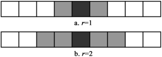
   2. In one-dimensional cellular automata, the neighborhood is usually determined by the radius r, and all cells within the distance r of a cell are considered neighbors of that cell.
      1. Neighbors of one-dimensional cellular automata:

      2. 

         
   3. In two-dimensional cellular automata, there are usually several types of neighborhoods:
      1. Von NeumanNeighborhoods
      2. MooreNeighborhoods
      3. Margolus Neighborhoods
         1. It treats one 2 *2 cell block at a time, while each of the first two types of neighborhoods is treated separately

         2. 

            
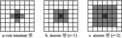
   4. Similarly, you can define neighborhoods for high-dimensional cellular automata over two dimensions
4. Status Update Rules
   1. A state transfer function that determines the state of a cell at the next moment based on its current state and the state of the cell in its neighborhood.
   2. Status update rules can be written as

      

      ，

      

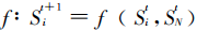
      _is a combination of neighborhood states at time t, called local mappings or local rules of cellular automata.

Characteristics of 2.2.2 Standard Cellular Automata

1. Discreteness: The space, time and state of cellular automata are discrete.
2. Homogeneity: Each cell in a cell space may have the same set of states, and the same rules governing the state changes of each cell.
3. Parallelism: Each cell in the cell space changes synchronously according to the state update rule, which is especially suitable for parallel computing. The state changes of each cell are independent and have no influence on each other.
4. Locality: The state of a cell at time t+1 is determined by the state of the cell at the current time t in the neighborhood around it with radius r. Therefore, there is locality in time and space.
5. High dimensionality: Cellular automata is an infinite-dimensional dynamic system.

Application of 1.3 Cellular Automation in Management System

Cellular automata have been widely used in various fields of social, economic, military and Natural Sciences

1. In sociology, cellular automata is used to study the emergence of political organizations, the sociality of individual behavior, and the spread of gossip.
2. In biology, it is used to study the growth mechanism and process simulation of tumor cells, the mechanism exploration of human brain, HIV infection process, self-organization, self-reproduction and other life phenomena, as well as cloning technology.
3. In computer science, cellular automata is considered a parallel computer for parallel computing.
4. In physics, in addition to the successful application of lattice gas cellular automata in fluid mechanics, cellular automata can also be used to simulate fields such as magnetic fields and electric fields, as well as heat diffusion, heat conduction and mechanical waves.
5. In military science, cellular automata is used to simulate military operations and understand the process of war.
6. In the field of management, domestic and foreign scholars begin to use cellular automata to explain and analyze various management phenomena, and to simulate the evolution of various management phenomena.

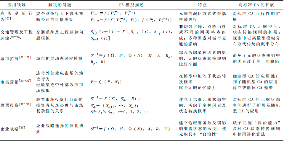
Application of Cellular Automation in Management Systems:



Part 2 Code

clear all;
close all;
pes_rate = 0.25;%%Pedestrian traffic (per second)	
car_rate = 0.2;%%Vehicle flow (per second)
car_avg_speed = 12;
w =21;%%Road Width
l = 9;%%Walkway width
road_len = 150;
pes_avg_speed = 1.2/0.6;%%Average speed of pedestrians, calculated by cell
pes_max_speed = 1.8/0.6;%%Maximum speed of pedestrians, calculated by cell
p_move = 0.7; %Moving Probability Without Advantage Channels						%★★★
r_adv = [4,2]; %Decision Spatial Range, 3 rows wide, Number of columns before and after each element of the matrix		%★★★
cat_avg_speed = 10/0.6;								%★★★What is this?
int_pes_num = ceil(w/pes_avg_speed*pes_rate);%%Initialize number of pedestrians
int_car_num = ceil(road_len/cat_avg_speed*car_rate);%%Initialize Number of Cars
num_l = floor(int_pes_num/2);
num_r = int_pes_num-num_l;
[space,ped_l,ped_r,v_space] = initialize_pes(w,l,num_l,num_r);%%Initialize pedestrian%%ped_l Top Pedestrian Sort,From top to bottom, ped_r Pedestrians below, moving from bottom to top

%
% ped_r.m(1)=8;									%★★★
% ped_r.n(1)=1;									%★★★
%
[l_id,r_id,v_l,v_r] = initialize_car(int_car_num,int_car_num,road_len,l);
% l_id = [];
% r_id = [80];									%★★★

car_vmax = 18.5;
pes_vmax = 1.8/0.6;
car_insert = [];
pes_insert = [];
sim_time = 40;									%★★★Is this the duration of the simulation?
add_car_num=0;
add_pes_num=0;
down_car_strat_id = l_id;
down_car_isfinished = zeros(size(l_id));
dowvcar_is_wait = zeros(size(l_id));
downcar_cross_time = zeros(size(l_id));
down_start_time = zeros(size(l_id));
up_car_start_id = r_id;
up_car_isfinished = zeros(size(r_id));
upcar_is_wait = zeros(size(r_id));
upcar_cross_time = zeros(size(r_id));
up_start_time = zeros(size(r_id));

down_cross_finish_time = [];
down_finish_time = [];
down_iswait_finished = [];
up_cross_finish_time = [];
up_finish_time = [];
up_iswait_finished = [];
down_finish_avg_v = [];
up_finish_avg_v = [];

down_pes_cross_time = zeros(size(ped_l.m));
down_pes_wait_time = zeros(size(ped_l.m));
up_pes_cross_time = zeros(size(ped_r.m));
up_pes_wait_time = zeros(size(ped_r.m));

down_pes_corss_time_finish= [];
down_pes_wait_time_finish= [];
up_pes_corss_time_finish= [];
up_pes_wait_time_finish= [];

%
% l_id = [58,18];								%★★★
%

%%Initialize Vehicle
figure(1);
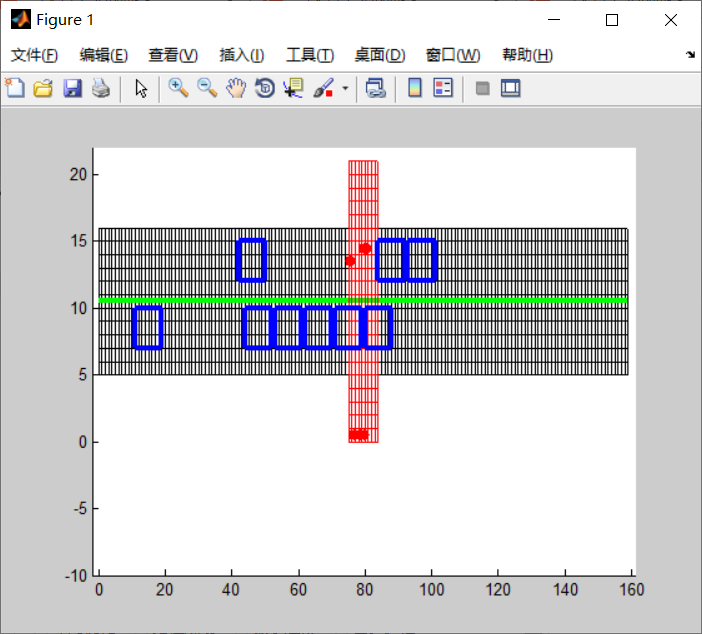
plot_map(ped_l,ped_r,space,20,l_id,r_id,road_len,l);
sim_min_num = 2;%Simulation time							%★★★

for min_ind = 1:sim_min_num
    [down_car_num,down_car_gen_inde] = get_car_num();
    [up_car_num,up_car_gen_inde] = get_car_num();
    for ss=1:3									%★★★
           [down_pes_num,down_time_start_id] = get_pes_num();
            [up_pes_num,up_time_start_id] = get_pes_num();
    
                l_id(id) = [];
                v_l(id) = [];
                dowvcar_is_wait(id) = [];
                downcar_cross_time(id) = [];
                down_start_time(id) = [];
                down_car_strat_id(id) = [];
            end
            %%Up Lane
            id = find(r_id<-4);							%★★★
            if ~isempty(id)
                up_cross_finish_time = [up_cross_finish_time,upcar_cross_time(id)];%%Pedestrian passage time
                up_finish_avg_v = [up_finish_avg_v,up_car_start_id(id)./(index-up_start_time(id))];
                up_finish_time = [up_finish_time,index-up_start_time(id)];%%Total travel time
                up_iswait_finished = [up_iswait_finished,upcar_is_wait(id)];
                %%Delete related data
                r_id(id) = [];
          
            if ismember(tt,up_time_start_id)%%Add Pedestrian Entry
                num = sum(up_time_start_id==tt);
                m=21;
                n = randperm(l,num);
                for add_ind = 1:num
                    ped_r.m(end+1) = m;
                    ped_r.n(end+1) = n(add_ind);
                    ped_r.p(end+1) =  n(add_ind)*w+m;
                    up_pes_cross_time(end+1) = 0;
                    up_pes_wait_time(end+1) = 0;
                    v_space(m, n(add_ind)) = rand(1)*pes_vmax;
                    space(m, n(add_ind))=1;
                end
            end
            
            
            
            figure(1);clf;
            plot_map(ped_l,ped_r,space,20,l_id,r_id,road_len,l);
            pause(0.6);
            drawnow;
        end
    end
end
norm_mean_time = l*0.6/car_avg_speed;
finish_car_num = numel(up_finish_avg_v)+numel(down_finish_avg_v);
road_capacity = 1650;
saturation = finish_car_num*60/1650;
fprintf('Average Vehicle Speed:%4.3f\n',mean([up_finish_avg_v,down_finish_avg_v]));
fprintf('Average delay time of vehicles at pedestrian crossings:%4.3f\n',mean([down_cross_finish_time-norm_mean_time,up_cross_finish_time-norm_mean_time]));
fprintf('Vehicle yield rate:%4.3f\n',sum([down_iswait_finished,up_iswait_finished])/numel([down_iswait_finished,up_iswait_finished]));
fprintf('saturation:%4.3f\n',saturation);
fprintf('Average pedestrian transit time:%4.3f\n',mean([down_pes_corss_time_finish,up_pes_corss_time_finish]));
fprintf('Average Pedestrian Waiting Time:%4.3f\n',mean([up_pes_wait_time_finish,down_pes_wait_time_finish]));

3 Simulation results

 

4 References

[1] Xue Luo Dimension.Simulation and Application of Pedestrian Flow in Bus Based on Cellular Automation [D]. East China Jiaotong University, 2020.

5 Code Download