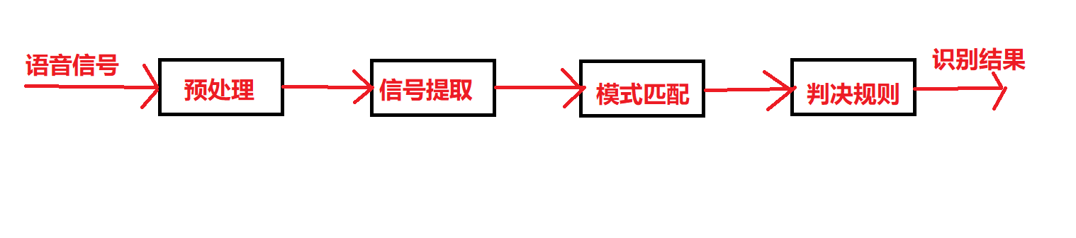
Speech feature recognition is an important aspect in the field of speech recognition, which is generally solved by the principle of pattern matching. The operation process of speech recognition is:

• Firstly, the speech to be recognized is transformed into an electrical signal and then input into the recognition system. After preprocessing, the speech feature signal is extracted by mathematical method. The extracted speech feature signal can be regarded as the pattern of the speech.
• Then, the speech model is compared with the known reference mode to obtain the best matching reference mode as the recognition result of the speech.
• The speech recognition process is shown in Figure 1.
  

Figure 1

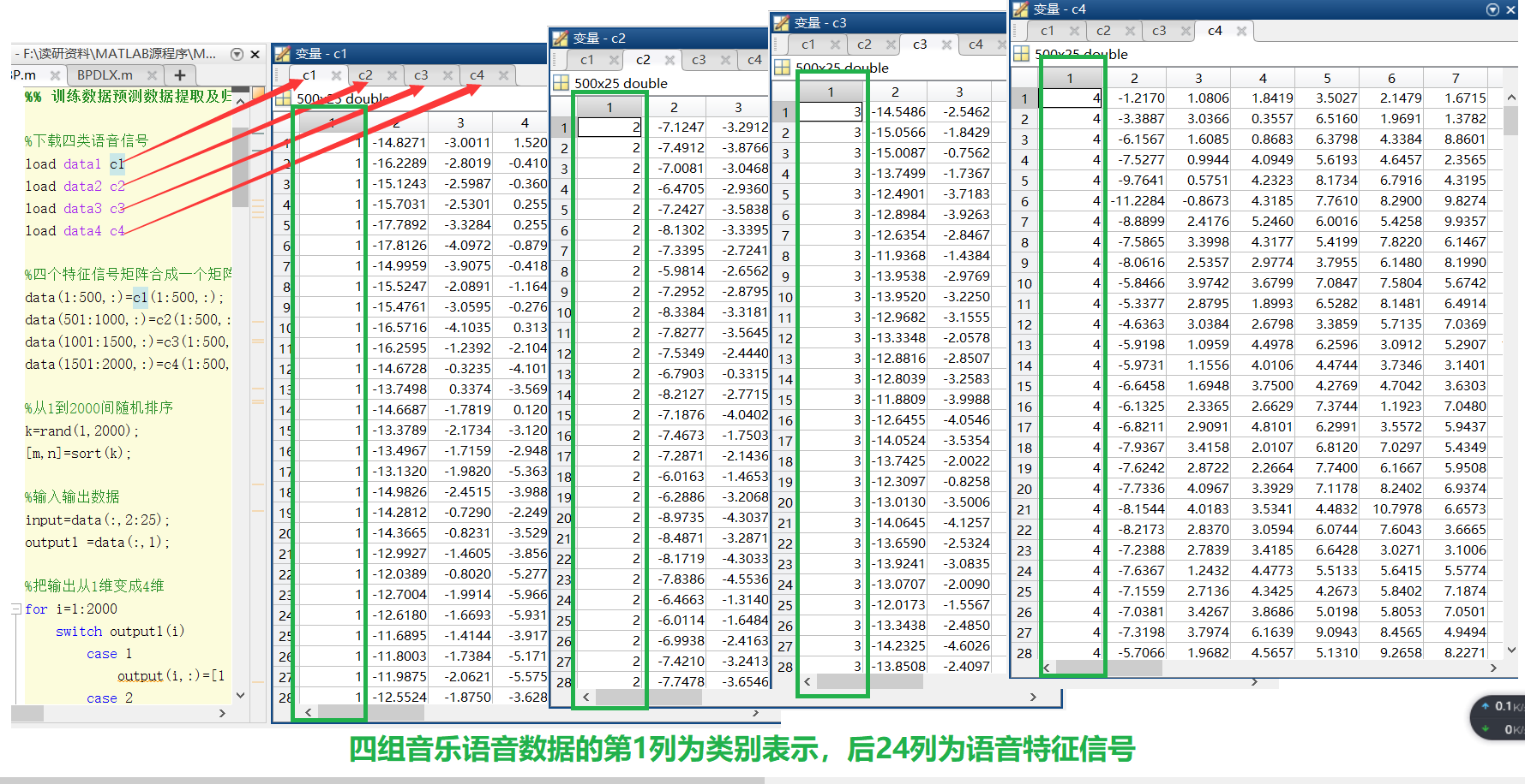
stay Baidu online disk attachment data - extraction code: qwer In, four kinds of music speech characteristic signals have been extracted. Different speech signals are identified with 1, 2, 3 and 4 respectively, and the extracted signals are stored in data1 mat , data2. mat , data3. mat , data4. In the mat database file, the data content is shown in Figure 2.
Each group of data is 25 dimensions, the first dimension is category identification, and the last 24 dimensions are speech feature signals. The four kinds of speech characteristic signals are combined into a group, 1500 groups of data are randomly selected as training data and 500 groups of data are used as test data, and the training data are normalized. Set the expected output value of each group of voice signals according to the voice category identification. For example, when the identification category is 1, the expected output vector is [1 0].

Figure 2

Before BP neural network prediction, the network must be trained first. Through training, the network has the ability of associative memory and prediction. The training process of BP neural network includes the following steps.

1. Network initialization. Determine the number of network input layer nodes n, hidden layer nodes l and output layer nodes m according to the system input and output sequence (X,Y), and initialize the connection weights between input layer, hidden layer and output layer neurons ω i j \omega _{{\rm{ij}}} ωij​, ω j k \omega _{{\rm{jk}}} ω jk, initialize hidden layer threshold a, output layer threshold b, given learning rate and neuron excitation function.
2. Hidden layer output calculation. According to the input vector X, the connection weight between the input layer and the hidden layer ω i j \omega _{{\rm{ij}}} ω ij, and the hidden layer threshold a, calculate the hidden layer output H.
3. Output layer output calculation. According to the hidden layer output H, connect the weight ω j k \omega _{{\rm{jk}}} ω jk ， and threshold b, calculate the BP neural network prediction output O
4. Error calculation. The network prediction error e is calculated according to the network prediction output O and the expected output Y.
5. Weight update. Update the network connection weight according to the network prediction error e ω i j \omega _{{\rm{ij}}} ωij​, ω j k \omega _{{\rm{jk}}} ωjk​
6. Threshold update. According to the network prediction error e, the network node thresholds A and B are updated.
7. Judge whether the algorithm iteration is over. If not, return to step 2.

The specific codes are as follows:

%% Clear environment variables
clc
clear

%% Training data prediction data extraction and normalization

%Download four types of voice signals
load data1 c1
load data2 c2
load data3 c3
load data4 c4
%Four characteristic signal matrices are combined into one matrix
data(1:500,:)=c1(1:500,:);
data(501:1000,:)=c2(1:500,:);
data(1001:1500,:)=c3(1:500,:);
data(1501:2000,:)=c4(1:500,:);

%Random sorting from 1 to 2000
k=rand(1,2000);
[m,n]=sort(k);  %n It is the number of 2000 randomly sorted

%Input / output data
input=data(:,2:25);  %Information of the last 24 locations of the original 2000 numbers
output1 =data(:,1);  %Information of the first position of the original 2000 numbers

%Change the output from 1D to 4D
for i=1:2000
    switch output1(i)
        case 1
            output(i,:)=[1 0 0 0];
        case 2
            output(i,:)=[0 1 0 0];
        case 3
            output(i,:)=[0 0 1 0];
        case 4
            output(i,:)=[0 0 0 1];
    end
end

%In accordance with the previously disrupted order, 1500 samples were randomly selected as training samples and 500 samples as prediction samples
input_train=input(n(1:1500),:)';
output_train=output(n(1:1500),:)';
input_test=input(n(1501:2000),:)';
output_test=output(n(1501:2000),:)';

%Input data normalization
[inputn,inputps]=mapminmax(input_train);  % Normalization principle formula: Xk=(Xk-Xmin)/(Xmax-Xmin)

%% Network structure initialization
%Network size initialization
innum=24;
midnum=25;
outnum=4;
 

%Weight initialization
w1=rands(midnum,innum);
b1=rands(midnum,1);
w2=rands(midnum,outnum);
b2=rands(outnum,1);

w2_1=w2;
w2_2=w2_1;
w1_1=w1;
w1_2=w1_1;

b1_1=b1;
b1_2=b1_1;
b2_1=b2;
b2_2=b2_1;

%Learning rate
xite=0.1;
alfa=0.01;

The BP neural network is trained with the training data, and the weight and threshold of the network are adjusted according to the network prediction error in the training process.

%% Network training
for ii=1:10
    E(ii)=0;
    for i=1:1:1500
       %% Network prediction output 
        x=inputn(:,i);
        % Hidden layer output
        for j=1:1:midnum
            I(j)=inputn(:,i)'*w1(j,:)'+b1(j);
            Iout(j)=1/(1+exp(-I(j)));
        end
        % Output layer output
        yn=w2'*Iout'+b2;
        
       %% Weight threshold correction
        %calculation error
        e=output_train(:,i)-yn;     
        E(ii)=E(ii)+sum(abs(e));
        
        %Calculate weight change rate
        dw2=e*Iout;
        db2=e';
        
        for j=1:1:midnum
            S=1/(1+exp(-I(j)));
            FI(j)=S*(1-S);
        end      
        for k=1:1:innum
            for j=1:1:midnum
                dw1(k,j)=FI(j)*x(k)*(e(1)*w2(j,1)+e(2)*w2(j,2)+e(3)*w2(j,3)+e(4)*w2(j,4));
                db1(j)=FI(j)*(e(1)*w2(j,1)+e(2)*w2(j,2)+e(3)*w2(j,3)+e(4)*w2(j,4));
            end
        end
           
        w1=w1_1+xite*dw1';
        b1=b1_1+xite*db1';
        w2=w2_1+xite*dw2';
        b2=b2_1+xite*db2';
        
        w1_2=w1_1;w1_1=w1;
        w2_2=w2_1;w2_1=w2;
        b1_2=b1_1;b1_1=b1;
        b2_2=b2_1;b2_1=b2;
    end
end

The trained BP neural network is used to classify speech characteristic signals, and the classification ability of BP neural network is analyzed according to the classification results.

%% Speech feature signal classification
inputn_test=mapminmax('apply',input_test,inputps);

for ii=1:1
    for i=1:500%1500
        %Hidden layer output
        for j=1:1:midnum
            I(j)=inputn_test(:,i)'*w1(j,:)'+b1(j);
            Iout(j)=1/(1+exp(-I(j)));
        end
        
        fore(:,i)=w2'*Iout'+b2;
    end
end

Analyze the experimental results. Draw the error diagram. Show accuracy.

%% Result analysis
%Find out what kind of data it belongs to according to the network output
for i=1:500
    output_fore(i)=find(fore(:,i)==max(fore(:,i)));
end

%BP Network prediction error
error=output_fore-output1(n(1501:2000))';



%Draw the classification diagram of predicted speech types and actual speech types
figure(1)
plot(output_fore,'r')
hold on
plot(output1(n(1501:2000))','b')
legend('Predicted speech category','Actual voice category')

%Draw the error diagram
figure(2)
plot(error)
title('BP Network classification error','fontsize',12)
xlabel('speech signal ','fontsize',12)
ylabel('Classification error','fontsize',12)

%print -dtiff -r600 1-4

k=zeros(1,4);  
%Find out the category of judgment errors
for i=1:500
    if error(i)~=0
        [b,c]=max(output_test(:,i));
        switch c
            case 1 
                k(1)=k(1)+1;
            case 2 
                k(2)=k(2)+1;
            case 3 
                k(3)=k(3)+1;
            case 4 
                k(4)=k(4)+1;
        end
    end
end

%Identify the individuals and of each category
kk=zeros(1,4);
for i=1:500
    [b,c]=max(output_test(:,i));
    switch c
        case 1
            kk(1)=kk(1)+1;
        case 2
            kk(2)=kk(2)+1;
        case 3
            kk(3)=kk(3)+1;
        case 4
            kk(4)=kk(4)+1;
    end
end

%Correct rate
rightridio=(kk-k)./kk

The final prediction effect is shown in Figure 3: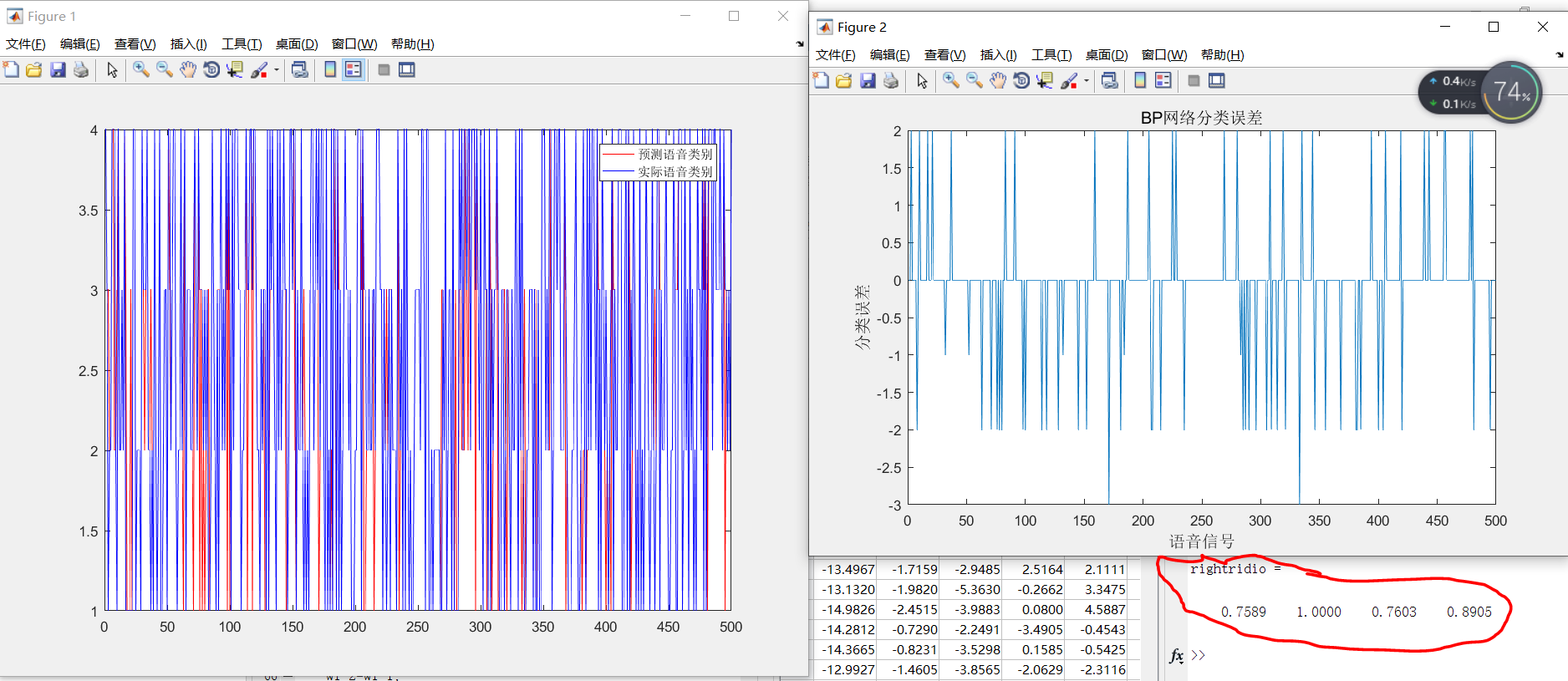

Figure 3

Seeing this content in the book, I want to write a blog to record it. If this blog is helpful to you, I hope I can praise, collect and pay attention to it. I will share high-quality blogs in the future. Thank you!