Summary of Classic Network Structure--MobileNet Series
MobileNet
mobilenet was proposed by Google.
Advantages: Small size, small computation, suitable for convolution neural network of mobile devices.
Classification/Target Detection/Semantic Segmentation can be implemented;
Miniaturization:
The convolution kernel is decomposed and replaced by the convolution kernels of 1xN and Nx1.
Using bottleneck structure, represented by SqueezeNet
Save in low precision floating point numbers, such as Deep Compression
Redundant convolution kernel pruning and Haffman coding.
mobilenet v1:
Referencing the traditional chain architecture such as VGNet, the network depth is improved by cascading convolution layers, thus improving the recognition accuracy. Disadvantages: Gradient diffusion.
(Gradient diffusion: chain rule of derivatives, where successive layers with a gradient less than 1 make the gradient smaller and smaller, resulting in a layer with a gradient of 0)
What problem do you want to solve?
In real-world scenarios, such as mobile devices, embedded devices, auto-driving, etc., computing power is limited, so the goal is to build a small and fast model.
What method was used to solve the problem (implementation):
In the MobleNet architecture, deep detachable convolution is used instead of traditional convolution.
In the MobleNet network, two shrinking superparameters are introduced: width factor and resolution multiplier. Width factor can reduce parameter and amount of calculation. Resolution only changes the amount of computation.
What problems still exist:
The structure of MobileNet v1 is too simple and is similar to that of a VGG cylinder, resulting in a low cost-effective network. If a subsequent series of ResNet is introduced, DenseNet and other structures (multiplex image features, add shortcuts) can greatly improve the performance of the network.
There are potential problems with deep convolution, and some kernel s have zero weights after training.
Deep separable convolution idea?
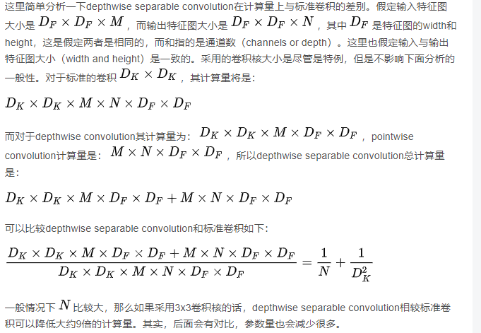
Essentially, the standard convolution is divided into two steps: the depthwise convolution and the pointwise convolution, whose inputs and outputs are the same.
depthwise convolution: Use a convolution kernel for each input channel individually.
pointwise convolution: 1 × 1 Convolution, which combines the output of the convolution of depthwise.
Most of MoblieNet's computations (about 95%) and parameters (75%) are in 1 × 1 In the convolution, most of the remaining parameters (about 24%) are in the full connection layer. Because the model is small, the means of regularization and data enhancement can be reduced, because small models are relatively difficult to fit.
Introduction
Convolutional neural network (CNN) has been widely used in the field of computer vision and has achieved good results. Figure 1 shows the performance of CNN in ImageNet competition in recent years. In order to pursue the accuracy of classification, the model depth becomes deeper and more complex. For example, the number of layers of deep residual network (ResNet) has reached 152.
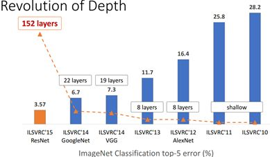
Figure 1 CNN performance on ImageNet (source: CVPR2017)
However, in some real applications such as mobile or embedded devices, such large and complex models are difficult to apply. First, the model is too large and it is facing the problem of insufficient memory. Second, these scenarios require low latency, or faster response. Imagine what terrible things would happen if the pedestrian detection system of an automobile was slow. Therefore, it is important to study small and efficient CNN models in these scenarios, at least for now, although hardware will become faster and faster in the future. The current research is summarized in two directions: one is to compress the trained complex models into small models; The second is to design and train small models directly. In any case, its goal is to reduce model size while increasing model speed while maintaining model performance (accuracy). The protagonist of this article, MobileNet, belongs to the latter, which is a compact and efficient CNN model recently proposed by Google that compromises between accuracy and latency. MobileNet is described in detail below.
Depthwise separable convolution
The basic unit of MobileNet is the depthwise separable convolution, which was previously used in the Inception model. Depth-level detachable convolution is actually a factorized convolution that can be broken down into two smaller operations: depthwise convolution and pointwise convolution, as shown in Figure 1. Depthwise convolution differs from standard convolution in that the convolution core for standard convolution is used on all input channels, while depthwise convolution uses different convolution cores for each input channel, that is, one convolution core corresponds to one input channel, so depthwise convolution is a depth level operation. The pointwise convolution is actually a normal convolution, but it uses a convolution core of 1x1. Two operations are more clearly shown in Figure 2. For depthwise separable convolution, it first convolutes different input channels using depthwise convolution, and then combines the above outputs using pointwise convolution. The overall effect is similar to a standard convolution, but the amount of calculation and model parameters will be greatly reduced.
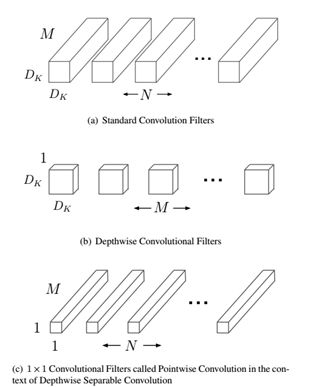
Figure 1 Depthwise separable convolution
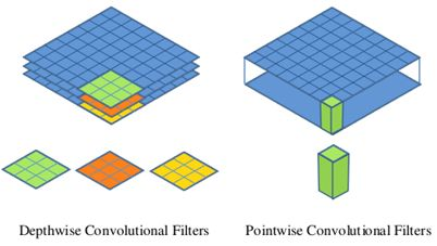
Figure 2 Depthwise convolution and pointwise convolution
MobileNet Network Architecture
The depthwise separable convolution was described earlier, which is a basic component of MobileNet, but batchnorm is added to the real application and the ReLU activation function is used, so the basic structure of the depthwise separable convolution is shown in Figure 3.
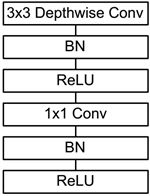
Figure 3 depthwise separable convolution with BN and ReLU
The network structure of MobileNet is shown in Table 1. First a standard convolution of 3x3, followed by a stacked depthwise separable convolution, and you can see that some of the depthwise convolution s are down-sampled by strides=2. Then use average pooling to turn feature into 1x1, add a full connection layer based on the size of the predicted category, and finally a soft Max layer. If depthwise is calculated separately
Convolution and pointwise convolution, the entire network has 28 layers (Avg Pool and Softmax are not counted here). We can also analyze the distribution of parameters and computations across the network, as shown in Table 2. You can see that the entire amount of computation is basically concentrated on the 1x1 convolution. If you are familiar with the underlying implementation of convolution, you should know that convolution is generally implemented by an im2col method, which requires memory reorganization. However, when the convolution core is 1x1, this is not needed, and the underlying layer can achieve faster implementation. The parameters are also mainly concentrated in 1x1 convolution, in addition to the full connection layer which accounts for a part of the parameters.
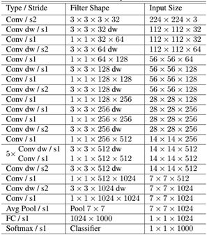
Table 1 Network structure of MobileNet
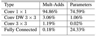
Table 2 Calculation and parameter distribution of MobileNet networks
How does MobileNet really work? This is compared with GoogleNet and VGG16, as shown in Table 3. MobileNet is slightly less accurate than VGG16, but better than GoogleNet. However, MobileNet has absolute advantages in terms of amount of computation and parameters.
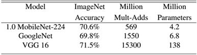
Table 3 Performance comparison of MobileNet with GoogleNet and VGG16
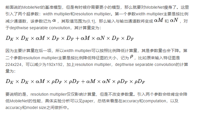
MobileNet Slim
The mobileNet benchmark model mentioned earlier, but sometimes you need a smaller model, so you need to lose weight to MobileNet. Two hyperparameters are introduced here: width multiplier and resolution multiplier.
TensorFlow implementation of MobileNet
The nn Library of TensorFlow has the depthwise convolution operator tf.nn.depthwise_conv2d, so MobileNet is easy to implement on TensorFlow:
class MobileNet(object):
    def __init__(self, inputs, num_classes=1000, is_training=True,
                 width_multiplier=1, scope="MobileNet"):
        """
        The implement of MobileNet(ref:https://arxiv.org/abs/1704.04861)
        :param inputs: 4-D Tensor of [batch_size, height, width, channels]
        :param num_classes: number of classes
        :param is_training: Boolean, whether or not the model is training
        :param width_multiplier: float, controls the size of model
        :param scope: Optional scope for variables
        """
        self.inputs = inputs
        self.num_classes = num_classes
        self.is_training = is_training
        self.width_multiplier = width_multiplier

        # construct model
        with tf.variable_scope(scope):
            # conv1
            net = conv2d(inputs, "conv_1", round(32 * width_multiplier), filter_size=3,
                         strides=2)  # ->[N, 112, 112, 32]
            net = tf.nn.relu(bacthnorm(net, "conv_1/bn", is_training=self.is_training))
            net = self._depthwise_separable_conv2d(net, 64, self.width_multiplier,
                                "ds_conv_2") # ->[N, 112, 112, 64]
            net = self._depthwise_separable_conv2d(net, 128, self.width_multiplier,
                                "ds_conv_3", downsample=True) # ->[N, 56, 56, 128]
            net = self._depthwise_separable_conv2d(net, 128, self.width_multiplier,
                                "ds_conv_4") # ->[N, 56, 56, 128]
            net = self._depthwise_separable_conv2d(net, 256, self.width_multiplier,
                                "ds_conv_5", downsample=True) # ->[N, 28, 28, 256]
            net = self._depthwise_separable_conv2d(net, 256, self.width_multiplier,
                                "ds_conv_6") # ->[N, 28, 28, 256]
            net = self._depthwise_separable_conv2d(net, 512, self.width_multiplier,
                                "ds_conv_7", downsample=True) # ->[N, 14, 14, 512]
            net = self._depthwise_separable_conv2d(net, 512, self.width_multiplier,
                                "ds_conv_8") # ->[N, 14, 14, 512]
            net = self._depthwise_separable_conv2d(net, 512, self.width_multiplier,
                                "ds_conv_9")  # ->[N, 14, 14, 512]
            net = self._depthwise_separable_conv2d(net, 512, self.width_multiplier,
                                "ds_conv_10")  # ->[N, 14, 14, 512]
            net = self._depthwise_separable_conv2d(net, 512, self.width_multiplier,
                                "ds_conv_11")  # ->[N, 14, 14, 512]
            net = self._depthwise_separable_conv2d(net, 512, self.width_multiplier,
                                "ds_conv_12")  # ->[N, 14, 14, 512]
            net = self._depthwise_separable_conv2d(net, 1024, self.width_multiplier,
                                "ds_conv_13", downsample=True) # ->[N, 7, 7, 1024]
            net = self._depthwise_separable_conv2d(net, 1024, self.width_multiplier,
                                "ds_conv_14") # ->[N, 7, 7, 1024]
            net = avg_pool(net, 7, "avg_pool_15")
            net = tf.squeeze(net, [1, 2], name="SpatialSqueeze")
            self.logits = fc(net, self.num_classes, "fc_16")
            self.predictions = tf.nn.softmax(self.logits)

    def _depthwise_separable_conv2d(self, inputs, num_filters, width_multiplier,
                                    scope, downsample=False):
        """depthwise separable convolution 2D function"""
        num_filters = round(num_filters * width_multiplier)
        strides = 2 if downsample else 1

        with tf.variable_scope(scope):
            # depthwise conv2d
            dw_conv = depthwise_conv2d(inputs, "depthwise_conv", strides=strides)
            # batchnorm
            bn = bacthnorm(dw_conv, "dw_bn", is_training=self.is_training)
            # relu
            relu = tf.nn.relu(bn)
            # pointwise conv2d (1x1)
            pw_conv = conv2d(relu, "pointwise_conv", num_filters)
            # bn
            bn = bacthnorm(pw_conv, "pw_bn", is_training=self.is_training)
            return tf.nn.relu(bn)
Full implementation can be found in GitHub.
summary
This paper briefly introduces the mobile end model MobileNet proposed by Google. The core of the model is to use a decomposable depthwise separable convolution, which can not only reduce the computational complexity of the model, but also greatly reduce the model size. In real mobile scenarios, networks like MobileNet will be the focus of ongoing research. Later we will introduce other mobile CNN models.
mobilenet v2:
mobileNet v2 introduced two major changes: Linear Bottleneck and Inverted Residual Blocks.
About Inverted Residual Blocks:
The MobileNet v2 architecture is based on inverted residual. It is essentially a residual network design. Traditional Residual block s are blocks with more channels at both ends and fewer middle channels.
The inverted residual designed in this paper is a block with fewer channel channels on both ends and more channels in the block. Deep detachable convolution is also preserved
About Linear Bottlenecks:
The area of interest remains non-zero after the ReLU and is approximated as a linear transformation.
ReLU maintains the integrity of input information, but is limited to low-dimensional subspaces where input features are located in the input space.
For low latitude spatial processing, the ReLU is approximated as a linear transformation.
v1 vs v2:
Same:
Depth-wise(DW) convolution and Point-wise (PW) convolution are used to extract features. Together, these two operations are called Depth-wise Separable Convolution, which was previously widely used in Xception. The advantage of this is that the time and space complexity of the convolution layer can be theoretically multiplied.
Difference:
2. v2 adds a new PW convolution before DW convolution. The reason for this is that DW convolution does not have the ability to change the number of channels on its own due to its computational nature. How many channels are given to it by the previous layer, how many channels will it output. So if the number of channels given by the previous layer is very small, DW can only extract features in low-dimensional space, so the effect is not good enough.
To improve this problem, v2 now matches a PW before each DW, which is specially designed for dimension increase and defines a dimension increase factor of 6, so that regardless of the number of input channels, after the first PW dimension increase, the DW will work hard in a relatively higher dimension.
v2 removes the activation function of the second pw, which the author calls Linear Bottleneck. The reason is that the authors believe that the activation function can effectively increase non-linearity in high-dimensional space, while in low-dimensional space it can destroy eigenvalues, which is not as good as linearity. The second main function of PW is dimension reduction, so according to the above theory, it is not appropriate to use ReLU6 after dimension reduction.
Summary of mobileNet v2:
The hardest thing to understand is that Linear Bottlenecks, which is very simple to implement, is that there is no ReLU6 after the second PW in the MobileNetv2 organization. For low latitude space, linear mapping preserves features, while non-linear mapping destroys them.
mobileNet v3
Efficient network building modules:
v3 is a model derived from neural architecture search, and the modules used internally are:
1. The V1 model introduces deep detachable convolution;
2. v2 introduces an inverse residual structure with linear bottlenecks;
3. Lightweight attention model based on squeeze and excitation structure;
Complementary search:
In network structure search, the author combines two technologies: resource-constrained NAS and NetAdapt, which are used to search each module of the network with limited computation and number of parameters, so they are called module-level search.