Introduction:
In learning and working, we can use the drawing function in MATLAB to process the data conveniently into the desired two-dimensional or three-dimensional graphics, so that we can analyze the data more intuitively. This paper mainly summarizes the use of two-dimensional drawing function.
Summary of two-dimensional drawing functions: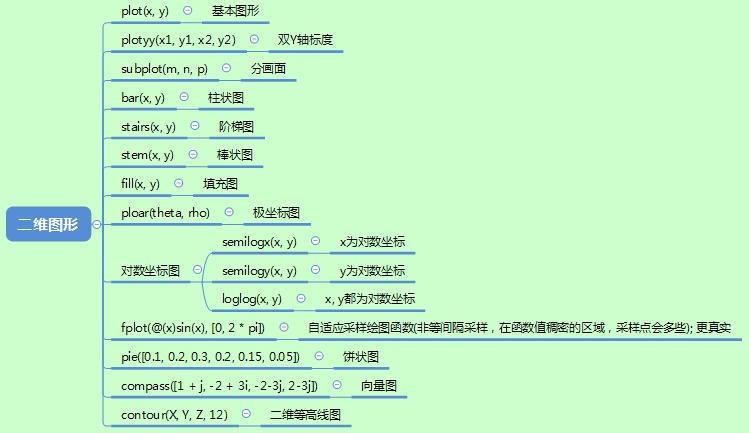

Code implementation:
[note]: each function provides at least one usage instance. When using, be careful to remove the comment symbol% in front of the code.

clear all; clc;
%--------------------------
% x = 0 : pi / 100 : 2 * pi;
% y = sin(x);
% plot(x, y);

%--------------------------
% t = -pi : pi / 100; pi;
% x = t .* cos(3 * t);
% y = t .* sin(t) .* sin(t);
% plot(x, y);

%--------------------------
% x = linspace(0, 2 * pi, 100);
% y = [sin(x); cos(x)];
% plot(x, y);

%--------------------------
% t = linspace(0, 2 * pi, 100);
% x = [t; t]';
% y = [sin(t); cos(t)]';
% plot(x, y);

%---------------------------
% x = 0 : pi / 100 : 2 * pi;
% y = exp(j * x);
% plot(y);

%---------------------------
% t = 0 : pi / 100 : 2 * pi;
% x = exp(j * t);
% y = [x; 2 * x; 3 * x]';
% plot(y);

%---------------------------
% x = linspace(0, 2 * pi, 100);
% plot(x, sin(x), ':', x, 2 * sin(x), '--', x, 3 * sin(x), '-.', x, 4 * sin(x));
% legend('sin(x)', '2sin(x)', '3sin(x)', '4sin(x)');

%-----------------------------
% x = 0 : pi / 100 : 2 * pi;
% y1 = 2 * exp(-0.5 * x);
% y2 = -2 * exp(-0.5 * x);
% y3 = 2 * exp(-0.5 * x) .* sin(2 * pi * x);
% plot(x, y1, '--', x, y2, '--', x, y3);
% % axis off;

%--------------------------------------------
% x1 = 0 : pi / 100 : 3 * pi;
% x2 = 0 : pi / 100 : 3 * pi;
% y1 = exp(-0.5 * x1) .* sin( 2 * pi * x1);
% y2 = 1.5 * exp(-0.1 * x2) .* sin(x2);
% plotyy(x1, y1, x2, y2);

%-------------------------------------------
% x = linspace(0, 10, 100);
% y = [];
% for x0 = x
%     if x0 < 4
%         y = [y, sqrt(x0)];
%     elseif x0 < 6
%         y = [y, 2];
%     elseif x0 < 8
%         y = [y, 5 - x0 / 2];
%     elseif x0 >= 8
%         y = [y, 1];
%     end
% end
% plot(x, y);
% axis([0, 10, 0, 2.5]);
% title('Piecewise function');
% xlabel('x'); ylabel('y');
% text(2, 1.3, 'y = x^{1/2}');
% text(4.5, 2.1, 'y = 2');
% text(7, 1.6, 'y = 5 - x / 2');
% text(8.5, 1.1, 'y = 1');

%--------------------------------
% x = 0 : pi / 100 : 2 * pi;
% y1 = sin(x);
% y2 = cos(x);
% subplot(1, 2, 1); plot(x, y1);
% title('sin(x)'); axis([0, 2 * pi, -1, 1]);
% 
% subplot(1, 2, 2); plot(x, y2);
% title('cos(x)'); axis([0, 2 * pi, -1, 1]);

%--------------------------------------------
% x = 0 : 0.35 : 7;
% y = exp(-0.5 * x);
% subplot(2, 2, 1); bar(x, y);
% subplot(2, 2, 2); stairs(x, y);
% subplot(2, 2, 3); stem(x, y);
% subplot(2, 2, 4); fill(x, y, 'b');

%--------------------------------------------
% theta = 0 : pi / 100 : 2 * pi;
% rho = theta;
% polar(theta, rho);

%-------------------------------------------
% x = 0 : 0.01 : 10;
% y = 10 * x .* x; % y = 10 * x^2
% subplot(2, 2, 1); plot(x, y);
% subplot(2, 2, 2); semilogx(x, y);
% subplot(2, 2, 3); semilogy(x, y);
% subplot(2, 2, 4); loglog(x, y);

%--------------------------------------------------------------
% subplot(2, 2, 1); fplot(@(x)sin(x), [0, 2 * pi]);
% subplot(2, 2, 2); fplot(@(x)[sin(x), cos(x)], [0, 2 * pi]);
% %Figure 3, 4 By contrast, Figure 3 shows more details.
% subplot(2, 2, 3); fplot(@(x)cos(tan(pi * x)), [-0.4, 1.4]);
% x = -0.4 : 0.01 : 1.4;
% subplot(2, 2, 4); plot(x, cos(tan(pi * x)));
%--------------------------------------------------------------
subplot(1, 2, 1); pie([0.1, 0.2, 0.3, 0.2, 0.15, 0.05]);
subplot(1, 2, 2); compass([1 + j, -2 + 3i, -2-3j, 2-3j]);