Introduction: _Using the basic functions in Paddle, ordinary linear and Logistic regression problems, especially the observation of the structure of network coefficients, are designed, which can then be used to modify the network.
Keywords: Paddle, Linear Regression, Logistics
_01 Basic Operations
_Tensor is the basic unit of operation under Paddle. This has more properties than the normal number, numpy matrix, such as shape, dtype, stop_gradient, etc.
1.1 Declare Tensor
_Using some initialization functions of paddle, it is easier to directly produce some special Tensor s.
_Below are all the properties of paddle, where ones, zeros, can be used to declare Tensor.
CPUPlace     CUDAPinnedPlace CUDAPlace    DataParallel Model        ParamAttr
Tensor       XPUPlace     __builtins__ __cached__   __doc__      __file__
__git_commit__ __loader__   __name__     __package__  __path__     __spec__
__version__  abs          acos         add          add_n        addmm
all          allclose     amp          any          arange       argmax
argmin       argsort      asin         assign       atan         batch
bernoulli    bmm          broadcast_shape broadcast_to callbacks    cast
ceil         cholesky     chunk        clip         common_ops_import compat
concat       conj         cos          cosh         create_parameter crop
cross        cumsum       dataset      device       diag         disable_static
dist         distributed  distribution divide       dot          empty
empty_like   enable_static equal        equal_all    erf          exp
expand       expand_as    eye          flatten      flip         floor
floor_divide floor_mod    flops        fluid        framework    full
full_like    gather       gather_nd    get_cuda_rng_state get_cudnn_version get_default_dtype
get_device   grad         greater_equal greater_than hapi         histogram
imag         in_dynamic_mode increment    incubate     index_sample index_select
inverse      io           is_compiled_with_cuda is_compiled_with_xpu is_empty     is_tensor
isfinite     isinf        isnan        jit          kron         less_equal
less_than    linspace     load         log          log10        log1p
log2         logical_and  logical_not  logical_or   logical_xor  logsumexp
masked_select matmul       max          maximum      mean         median
meshgrid     metric       min          minimum      mm           mod
monkey_patch_math_varbase monkey_patch_variable multinomial  multiplex    multiply     mv
nn           no_grad      nonzero      norm         normal       not_equal
numel        ones         ones_like    onnx         optimizer    os
paddle       pow          prod         rand         randint      randn
randperm     rank         reader       real         reciprocal   regularizer
remainder    reshape      reshape_     reverse      roll         round
rsqrt        save         scale        scatter      scatter_     scatter_nd
scatter_nd_add seed         set_cuda_rng_state set_default_dtype set_device   set_printoptions
shape        shard_index  sign         sin          sinh         slice
sort         split        sqrt         square       squeeze      squeeze_
stack        standard_normal stanh        static       std          strided_slice
subtract     sum          summary      sysconfig    t            tanh
tanh_        tensor       text         tile         to_tensor    topk
trace        transpose    tril         triu         unbind       uniform
unique       unsqueeze    unsqueeze_   unstack      utils        var
1.1. 1 Declare Tensor
x1 = paddle.zeros([2,2], dtype='int64')
x2 = paddle.ones([2,2], dtype='float64')

x3 = x1 + x2
print(x3)
Tensor(shape=[2, 2], dtype=int64, place=CPUPlace, stop_gradient=True,
[[1, 1],
[1, 1]])
_From the results above, for different data types (float64, int64), the final result is converted to the type of int64.
_02 Linear Regression
2.1 Defining a data model
_We use numpy to define a set of data, 13 of which are each, and for example, all but the first number is filled with 0. This set of data is y = 2 * x + 1, but the program is unknown. We then use this set of data to train to see if a strong neural network can train a model to fit this function. Finally, a prediction data is defined, which is used as the X-input at the end of the training to see if the predictions are close to the correct values.
2.1. 1 Builder Function
x_data = array([[i]+[0]*12 for i in range(1,6)]).astype('float32')
y_data = array([[i*2+1] for i in range(1,6)]).astype('float32')
test_data = array([[6]+[0]*12]).astype('float32')
print(x_data, "\n",  y_data, "\n",  test_data)
2.1. 2 Build results
x_data = array([[i]+[0]*12 for i in range(1,6)]).astype('float32')
y_data = array([[i*2+1] for i in range(1,6)]).astype('float32')
test_data = array([[6]+[0]*12]).astype('float32')
print(x_data, "\n\n",  y_data, "\n\n",  test_data)
[[1. 0. 0. 0. 0. 0. 0. 0. 0. 0. 0. 0. 0.]
[2. 0. 0. 0. 0. 0. 0. 0. 0. 0. 0. 0. 0.]
[3. 0. 0. 0. 0. 0. 0. 0. 0. 0. 0. 0. 0.]
[4. 0. 0. 0. 0. 0. 0. 0. 0. 0. 0. 0. 0.]
[5. 0. 0. 0. 0. 0. 0. 0. 0. 0. 0. 0. 0.]]
[[ 3.]
[ 5.]
[ 7.]
[ 9.]
[11.]]
[[6. 0. 0. 0. 0. 0. 0. 0. 0. 0. 0. 0. 0.]]
2.2 Building Linear Networks
2.2. 1 Network Structure
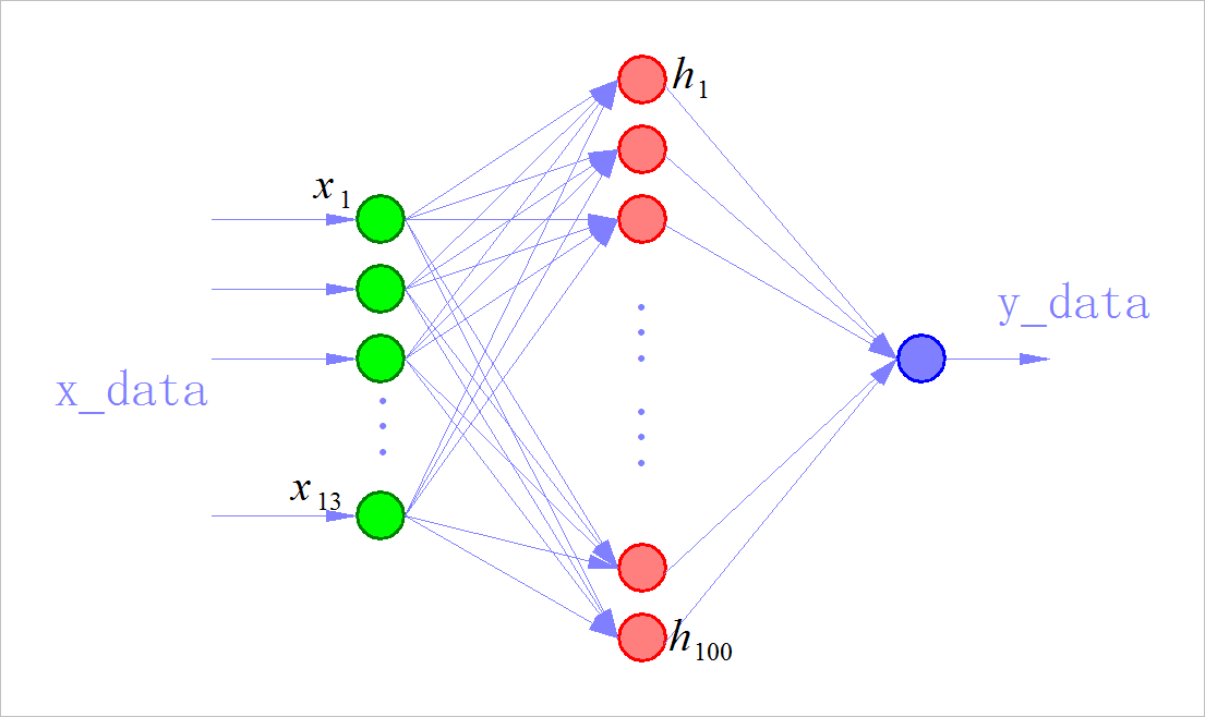
_Defines a simple linear network, which is very simple and structured as:
[Input Layer][Hidden Layer][Activation Function][Output Layer]
_More specifically, a fully connected layer with an output size of 100, followed by an activation function ReLU and a fully connected layer with an output size of 1, constructs a very simple network.
_The shape of the input layer is defined here as 13, because each data in the Boston House Price Data Set has 13 attributes, and the datasets we customize later are designed to fit this dimension.
2.2. 2 Define a linear network
(1) Network structure
net = paddle.nn.Sequential(
    paddle.nn.Linear(13,100),
    paddle.nn.ReLU(),
    paddle.nn.Linear(100,1),
)

optimizer = paddle.optimizer.SGD(learning_rate=0.01, parameters=net.parameters())
_Next comes the definition of the optimization method used in training, where the random gradient descent optimization method is used. PaddlePaddle provides a number of optimization function interfaces. In addition to the random gradient descent (SGD) method used in this project, Momentum, Adagrad, Adagrad, and so on, readers can use different optimization methods for their own project needs.
(2) Define the loss function
_Because this project is a linear regression task, we used the Square Difference Loss function in our training. Because paddle. Nn. Function. Square_ Error_ Cost is asking for a Batch loss, so we're also asking for an average. PaddlePaddle provides many interfaces for loss functions, such as the cross-entropy loss function paddle.nn.CrossEntropyLoss.
_During the training process, we can see that the output loss value is decreasing, which proves that our model is convergent.
import paddle
import paddle.nn.functional as F
from paddle import to_tensor as TT
from paddle.nn.functional import square_error_cost as sqrc
net = paddle.nn.Sequential(
    paddle.nn.Linear(13,100),
    paddle.nn.ReLU(),
    paddle.nn.Linear(100,1),
)

optimizer = paddle.optimizer.SGD(learning_rate=0.01, parameters=net.parameters())

inputs = TT(x_data)
labels = TT(y_data)

for pass_id in range(10):
    out = net(inputs)
    loss = paddle.mean(sqrc(out, labels))

    loss.backward()
    optimizer.step()
    optimizer.clear_grad()

    print("pass: %d, Cost:%0.5f"%(pass_id, loss))
pass: 0, Cost:71.86705
pass: 1, Cost:30.57855
pass: 2, Cost:11.62621
pass: 3, Cost:1.53674
pass: 4, Cost:0.02941
pass: 5, Cost:0.01128
pass: 6, Cost:0.01104
pass: 7, Cost:0.01081
pass: 8, Cost:0.01058
pass: 9, Cost:0.01036
_After the training, we used the forecasting program obtained from the cloning main program above to predict the forecasting data that we just defined. When we define the data above, the rule y = 2 * x + 1 is satisfied, so when x is 6, y should be 13, and the final output should be close to 13.
2.2. 3 Network Prediction
predict_inputs = TT(test_data)
result = net(predict_inputs)

print('x=%0.3f, y=%0.5f'%(test_data.flatten()[0], result))
x=6.000, y=13.15371
2.3 Network parameters
Where are the parameters of the linear model ahead?
2.3. 1 All parameter types
parms = net.parameters()
print(type(parms))
print(len(parms))

_=[print(type(parms[i])) for i in range(len(parms))]
<class 'list'>
4
<class 'paddle.fluid.framework.ParamBase'>
<class 'paddle.fluid.framework.ParamBase'>
<class 'paddle.fluid.framework.ParamBase'>
<class 'paddle.fluid.framework.ParamBase'>
2.3. 2 First parameter
_The first parameter is the matrix input to the hidden layer, shape = (13,10)
print(parms[0].numpy())
[[-0.075387 0.5339514 -0.5040579 0.21901496 0.34557822 -0.11829474
-0.00709895 0.37773132 0.8291067 0.7896065 ]
[ 0.2871285 -0.43426144 -0.15709287 -0.1772753 0.00291133 0.097902
0.03845656 -0.20523474 -0.37873447 0.09981477]
[ 0.10757929 -0.01285398 -0.24694431 0.07925624 -0.18733147 0.08271486
0.37385654 -0.22516277 0.29894334 -0.49872464]
[ 0.31193787 0.27885395 -0.3627605 0.116359 -0.06722078 -0.33219916
0.27342808 -0.24131414 0.42575645 0.05287254]
[-0.4429462 -0.2931974 0.09456986 -0.2963 -0.3600033 -0.24172312
0.05790824 -0.28486678 -0.44249436 0.13542217]
[ 0.49579376 -0.3068263 0.4475448 -0.21869034 -0.22201723 0.14771122
-0.26021212 -0.49464276 -0.0877367 -0.22605684]
[ 0.43755406 -0.43096933 0.3386714 -0.28694224 -0.03674829 0.39764756
-0.3881266 0.35218292 0.00819886 0.04092628]
[ 0.26412088 -0.05456609 -0.25517958 0.01412582 0.29454744 -0.3844456
0.24271363 0.26424062 0.35327762 0.39541048]
[-0.0133011 0.24380505 0.42668605 -0.19451535 -0.31308573 0.33640432
0.40896732 0.13685054 0.38675517 -0.06989819]
[ 0.13358372 -0.36512688 0.06258923 -0.29652268 0.29847944 0.04026729
-0.23680806 -0.13740104 0.40020412 0.50566524]
[-0.47494102 -0.32276535 -0.03033391 -0.33728325 0.32518142 -0.31474313
0.24827117 -0.42601836 -0.44340318 -0.3654582 ]
[-0.09328851 -0.48388985 -0.16385913 -0.18592414 0.06326699 -0.4801174
0.48408395 0.20635891 0.14444119 0.08807671]
[ 0.21163589 -0.02607039 0.36036986 -0.11807913 -0.2828287 0.23282737
-0.23758212 -0.41061205 0.1697821 0.25588465]]
2.3. 3Second parameter
_The second parameter is the offset of all cryptogenic neurons, shape=(1,10)
print(parms[1].numpy())
[ 0. 0.04476326 0. 0.04997304 -0.00701768 -0.07669634
-0.01661819 0.10008517 0.1378215 0.12973393]
2.3. 4 Third parameter
_The third parameter outputs the weights of the neurons in the form of (10,1)
print(parms[2].numpy())
[[-0.54290414]
[ 0.4281348 ]
[ 0.6710895 ]
[ 0.3250693 ]
[ 0.10694236]
[-0.6338133 ]
[-0.1300693 ]
[ 0.626347 ]
[ 0.9877776 ]
[ 0.93352455]]
2.3. 5Fourth parameter
The fourth parameter is the offset of the output neuron:
print(parms[3].numpy())
[0.17823167]
2.4 Network Performance
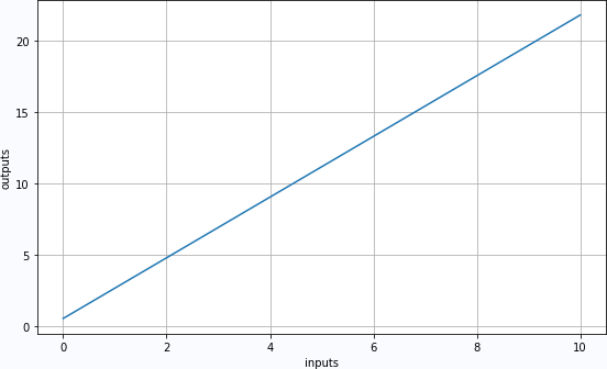
2.4. 1 Input and Output
td2 = TT(array([[i]+[0]*12 for i in linspace(0,10,100)]).astype('float32'))
prd2 = net(td2)

plt.figure(figsize=(8,5))
plt.plot(td2.numpy().T[0], prd2.numpy().T[0])
plt.xlabel("inputs")
plt.ylabel("outputs")
plt.grid(True)
plt.tight_layout()
plt.show()
2.4.2 LMS estimates W,b
x = td2.numpy().T[0]
y = prd2.numpy().T[0]
W = linalg.inv(dot(x[:,newaxis],x[newaxis,:])+eye(len(y))*0.1).dot(x).dot(y)
B = mean(y-W*x)
print('W:%0.5f'%W, "\n",  'b:%0.5f'%B)
W:2.20889
b:0.13555
_03 Logistic Regression
3.1 Network Definition
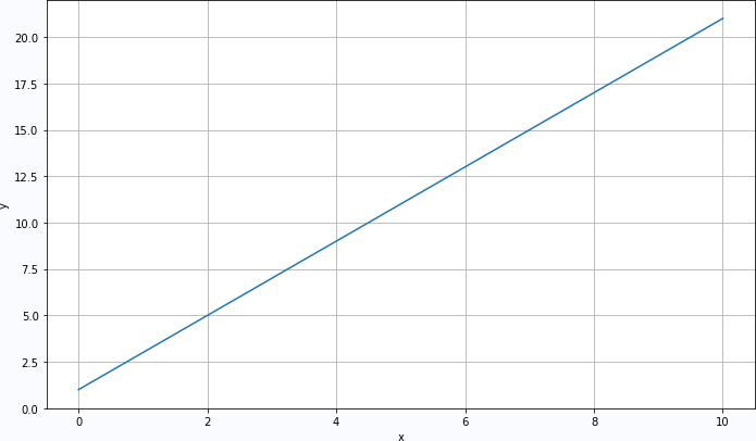
Increase data volume:
t = linspace(0, 10, 100)
x_data = array([[i]+[0]*12 for i in t]).astype('float32')
y_data = array([[i*2+1] for i in t]).astype('float32')
test_data = array([[6]+[0]*12]).astype('float32')

plt.plot(t, y_data.flatten())
plt.xlabel("x")
plt.ylabel("y")
plt.grid(True)
plt.tight_layout()
plt.show()

 #------------------------------------------------------------

net = paddle.nn.Sequential(
    paddle.nn.Linear(13,200),
    paddle.nn.Sigmoid(),
    paddle.nn.Linear(200,1),
)

optimizer = paddle.optimizer.SGD(learning_rate=0.005, parameters=net.parameters())

inputs = TT(x_data)
labels = TT(y_data)

for pass_id in range(10000):
    out = net(inputs)
    loss = paddle.mean(sqrc(out, labels))

    loss.backward()
    optimizer.step()
    optimizer.clear_grad()

    if pass_id % 1000 == 0:
        print("pass: %d, Cost:%0.5f"%(pass_id, loss))
3.2 Training Result
3.2. 1 Input data
3.2. 2 Training process
pass: 0, Cost:163.94566
pass: 1000, Cost:0.14547
pass: 2000, Cost:0.08274
pass: 3000, Cost:0.05948
pass: 4000, Cost:0.04697
pass: 5000, Cost:0.03904
pass: 6000, Cost:0.03352
pass: 7000, Cost:0.02943
pass: 8000, Cost:0.02627
pass: 9000, Cost:0.02374
3.2. 3 Prediction results
td2 = TT(array([[i]+[0]*12 for i in linspace(0,10,100)]).astype('float32'))

prd2 = net(td2)

plt.figure(figsize=(8,5))
plt.plot(td2.numpy().T[0], prd2.numpy().T[0])
plt.xlabel("inputs")
plt.ylabel("outputs")
plt.grid(True)
plt.tight_layout()
plt.show()

 #------------------------------------------------------------
x = td2.numpy().T[0]
y = prd2.numpy().T[0]
W = linalg.inv(dot(x[:,newaxis],x[newaxis,:])+eye(len(y))*0.1).dot(x).dot(y)
B = mean(y-W*x)
print('W:%0.5f'%W, "\n",  'b:%0.5f'%B)
3.2. 4 Forecast results
td2 = TT(array([[i]+[0]*12 for i in linspace(0,10,100)]).astype('float32'))

prd2 = net(td2)

plt.figure(figsize=(10,6))
plt.plot(td2.numpy().T[0], prd2.numpy().T[0])
plt.xlabel("inputs")
plt.ylabel("outputs")
plt.grid(True)
plt.tight_layout()
plt.show()

 #------------------------------------------------------------
x = td2.numpy().T[0]
y = prd2.numpy().T[0]
W = linalg.inv(dot(x[:,newaxis],x[newaxis,:])+eye(len(y))*0.1).dot(x).dot(y)
B = mean(y-W*x)
print('W:%0.5f'%W, "\n",  'b:%0.5f'%B)
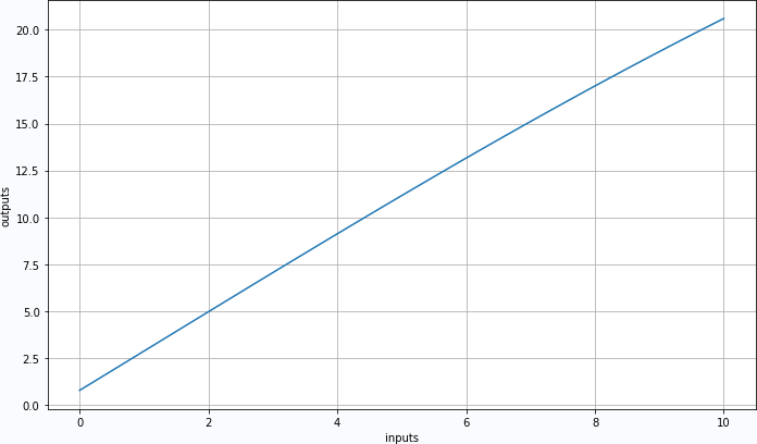
_Linear parameter results:
W:2.14812
b:0.25936
_total_knot_
_Using the basic functions in Paddle, ordinary linear and Logistic regression problems, especially the observation of the structure of network coefficients, are designed, which can then be used to modify the network.
Related chart links: