Data set partition

Firstly, the data set is divided into training set, verification set and test set, marked as X,y, Xval,yval and Xtest,ytest. The content of data set division can be seen This blog.

Data visualization

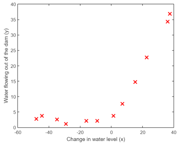
The first step of Wu Enda's routine operation is data visualization. Here, only the training set is visualized:

% Load from ex5data1: 
% You will have X, y, Xval, yval, Xtest, ytest in your environment
load ('ex5data1.mat');
% m = Number of examples
m = size(X, 1);

% Plot training data
figure;
plot(X, y, 'rx', 'MarkerSize', 10, 'LineWidth', 1.5);
xlabel('Change in water level (x)');
ylabel('Water flowing out of the dam (y)');

Cost gradient function

Linear regression is the most basic machine learning algorithm, and its cost and gradient formula are believed to be large 🔥 No stranger. The cost function is
J ( θ ) = 1 2 m ∑ i = 1 m ( θ 0 x 0 ( i ) + θ 1 x 1 ( i ) + ⋯ + θ n x n ( i ) − y ( i ) ) 2 + λ 2 m ∑ j = 1 n θ j 2 J(\theta)=\frac{1}{2m}\sum_{i=1}^m(\theta_0x_0^{(i)}+\theta_1x_1^{(i)}+\cdots+\theta_nx_n^{(i)}-y^{(i)})^2+\frac{\lambda}{2m}\sum_{j=1}^n\theta_j^2 J(θ)=2m1​i=1∑m​(θ0​x0(i)​+θ1​x1(i)​+⋯+θn​xn(i)​−y(i))2+2mλ​j=1∑n​θj2​
Gradient is
∂ J ( θ ) ∂ θ j = 1 m ∑ i = 1 m x j ( i ) ( θ 0 x 0 ( i ) + θ 1 x 1 ( i ) + ⋯ + θ n x n ( i ) − y ( i ) ) + λ m θ j \frac{\partial J(\theta)}{\partial \theta_j}=\frac{1}{m}\sum_{i=1}^m x_j^{(i)}(\theta_0x_0^{(i)}+\theta_1x_1^{(i)}+\cdots+\theta_nx_n^{(i)}-y^{(i)})+\frac{\lambda}{m}\theta_j ∂θj​∂J(θ)​=m1​i=1∑m​xj(i)​(θ0​x0(i)​+θ1​x1(i)​+⋯+θn​xn(i)​−y(i))+mλ​θj​
The vectorization process is also quite simple. Pay attention θ 0 \theta_0 θ 0 # just don't participate in regularization. I'll go directly to the code:

function [J, grad] = linearRegCostFunction(X, y, theta, lambda)
%LINEARREGCOSTFUNCTION Compute cost and gradient for regularized linear 
%regression with multiple variables
%   [J, grad] = LINEARREGCOSTFUNCTION(X, y, theta, lambda) computes the 
%   cost of using theta as the parameter for linear regression to fit the 
%   data points in X and y. Returns the cost in J and the gradient in grad

% Initialize some useful values
m = length(y); % number of training examples

% You need to return the following variables correctly 
J = 0;
grad = zeros(size(theta));

% ====================== YOUR CODE HERE ======================
% Instructions: Compute the cost and gradient of regularized linear 
%               regression for a particular choice of theta.
%
%               You should set J to the cost and grad to the gradient.
%

h=X*theta;
J=sum((h-y).^2)/(2*m);
J=J+(lambda/(2*m))*(sum(theta.^2)-theta(1)^2);

grad=X'*(h-y)/m;
tmp=grad(1);
grad=grad+(lambda/m)*theta;
grad(1)=tmp;

% =========================================================================

grad = grad(:);

end

solve

The solution process is very simple. Just call the cost gradient function we wrote. Wu Enda directly provided the code:

function [theta] = trainLinearReg(X, y, lambda)
%TRAINLINEARREG Trains linear regression given a dataset (X, y) and a
%regularization parameter lambda
%   [theta] = TRAINLINEARREG (X, y, lambda) trains linear regression using
%   the dataset (X, y) and regularization parameter lambda. Returns the
%   trained parameters theta.
%

% Initialize Theta
initial_theta = zeros(size(X, 2), 1); 

% Create "short hand" for the cost function to be minimized
costFunction = @(t) linearRegCostFunction(X, y, t, lambda);

% Now, costFunction is a function that takes in only one argument
options = optimset('MaxIter', 200, 'GradObj', 'on');

% Minimize using fmincg
theta = fmincg(costFunction, initial_theta, options);

end

Linear fitting

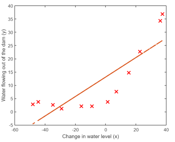
First, we try to use a straight line (one eigenvalue and two parameters) to fit, and the effect is certainly not good. This is the result:

Draw learning curve

Obviously, the problem of under fitting appears above, and we can confirm this judgment through its learning curve. The function for calculating the training cost and verification cost is basically the same as the cost function, but does not contain the regular term. Then calculate the cost while changing the size of the training set:

function [error_train, error_val] = ...
    learningCurve(X, y, Xval, yval, lambda)
%LEARNINGCURVE Generates the train and cross validation set errors needed 
%to plot a learning curve
%   [error_train, error_val] = ...
%       LEARNINGCURVE(X, y, Xval, yval, lambda) returns the train and
%       cross validation set errors for a learning curve. In particular, 
%       it returns two vectors of the same length - error_train and 
%       error_val. Then, error_train(i) contains the training error for
%       i examples (and similarly for error_val(i)).
%
%   In this function, you will compute the train and test errors for
%   dataset sizes from 1 up to m. In practice, when working with larger
%   datasets, you might want to do this in larger intervals.
%

% Number of training examples
m = size(X, 1);

% You need to return these values correctly
error_train = zeros(m, 1);
error_val   = zeros(m, 1);

% ====================== YOUR CODE HERE ======================
% Instructions: Fill in this function to return training errors in 
%               error_train and the cross validation errors in error_val. 
%               i.e., error_train(i) and 
%               error_val(i) should give you the errors
%               obtained after training on i examples.
%
% Note: You should evaluate the training error on the first i training
%       examples (i.e., X(1:i, :) and y(1:i)).
%
%       For the cross-validation error, you should instead evaluate on
%       the _entire_ cross validation set (Xval and yval).
%
% Note: If you are using your cost function (linearRegCostFunction)
%       to compute the training and cross validation error, you should 
%       call the function with the lambda argument set to 0. 
%       Do note that you will still need to use lambda when running
%       the training to obtain the theta parameters.
%
% Hint: You can loop over the examples with the following:
%
%       for i = 1:m
%           % Compute train/cross validation errors using training examples 
%           % X(1:i, :) and y(1:i), storing the result in 
%           % error_train(i) and error_val(i)
%           ....
%           
%       end
%

% ---------------------- Sample Solution ----------------------

for i=1:m
    tmpX=X(1:i,:);
    tmpy=y(1:i);
    [theta]=trainLinearReg(tmpX, tmpy, lambda);
    [error_train(i)]=linearRegCostFunction(tmpX,tmpy,theta,0);
    [error_val(i)]=linearRegCostFunction(Xval,yval,theta,0);
end




% -------------------------------------------------------------

% =========================================================================

end

lambda = 0;
[error_train, error_val] = learningCurve([ones(m, 1) X], y, [ones(size(Xval, 1), 1) Xval], yval, lambda);

plot(1:m, error_train, 1:m, error_val);
title('Learning curve for linear regression')
legend('Train', 'Cross Validation')
xlabel('Number of training examples')
ylabel('Error')
axis([0 13 0 150])

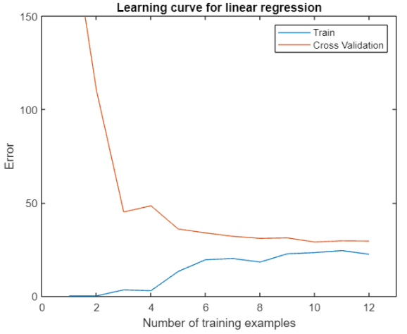
A better approach is to randomly select examples from the training set and from the cross validation set. Then, the randomly selected training set is used to learn the parameters, and the parameters are evaluated on the randomly selected training set and cross validation set. Repeat the above steps several times (such as 50 times), and use the average error to determine the training error and cross validation error of the example, so as to obtain a smoother curve.

Polynomial fitting

Obviously, we can't be satisfied with fitting with a straight line. We should try to use polynomials, which should also be used when fitting with polynomials Feature scaling . Feature scaling in ex1 Similar functions have been implemented. The code provided by Wu Enda is also similar, but high-level functions are called:

function [X_norm, mu, sigma] = featureNormalize(X)
%FEATURENORMALIZE Normalizes the features in X 
%   FEATURENORMALIZE(X) returns a normalized version of X where
%   the mean value of each feature is 0 and the standard deviation
%   is 1. This is often a good preprocessing step to do when
%   working with learning algorithms.

mu = mean(X);
X_norm = bsxfun(@minus, X, mu);

sigma = std(X_norm);
X_norm = bsxfun(@rdivide, X_norm, sigma);


% ============================================================

end

We implement the function of generating high-order terms:

function [X_poly] = polyFeatures(X, p)
%POLYFEATURES Maps X (1D vector) into the p-th power
%   [X_poly] = POLYFEATURES(X, p) takes a data matrix X (size m x 1) and
%   maps each example into its polynomial features where
%   X_poly(i, :) = [X(i) X(i).^2 X(i).^3 ...  X(i).^p];
%


% You need to return the following variables correctly.
X_poly = zeros(numel(X), p);

% ====================== YOUR CODE HERE ======================
% Instructions: Given a vector X, return a matrix X_poly where the p-th 
%               column of X contains the values of X to the p-th power.
%
% 

for i=1:p
    X_poly(:,i)=X.^i;
end



% =========================================================================

end

p = 8;

% Map X onto Polynomial Features and Normalize
X_poly = polyFeatures(X, p);
[X_poly, mu, sigma] = featureNormalize(X_poly);  % Normalize
X_poly = [ones(m, 1), X_poly];                   % Add Ones

% Map X_poly_test and normalize (using mu and sigma)
X_poly_test = polyFeatures(Xtest, p);
X_poly_test = X_poly_test-mu; % uses implicit expansion instead of bsxfun
X_poly_test = X_poly_test./sigma; % uses implicit expansion instead of bsxfun
X_poly_test = [ones(size(X_poly_test, 1), 1), X_poly_test];         % Add Ones

% Map X_poly_val and normalize (using mu and sigma)
X_poly_val = polyFeatures(Xval, p);
X_poly_val = X_poly_val-mu; % uses implicit expansion instead of bsxfun
X_poly_val = X_poly_val./sigma; % uses implicit expansion instead of bsxfun
X_poly_val = [ones(size(X_poly_val, 1), 1), X_poly_val];           % Add Ones

fprintf('Normalized Training Example 1:\n');

Solve again

% Train the model
lambda = 0;
[theta] = trainLinearReg(X_poly, y, lambda);
% Plot training data and fit
plot(X, y, 'rx', 'MarkerSize', 10, 'LineWidth', 1.5);
plotFit(min(X), max(X), mu, sigma, theta, p);
xlabel('Change in water level (x)');
ylabel('Water flowing out of the dam (y)');
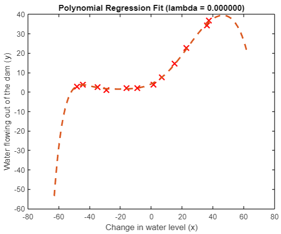
title (sprintf('Polynomial Regression Fit (lambda = %f)', lambda));

Because there are regular parameters here λ \lambda λ Set to 0, obviously our model is over fitted:

This can also be judged from its learning curve:

plot(1:m, error_train, 1:m, error_val);
title(sprintf('Polynomial Regression Learning Curve (lambda = %f)', lambda));
xlabel('Number of training examples')
ylabel('Error')
axis([0 13 0 100])
legend('Train', 'Cross Validation')

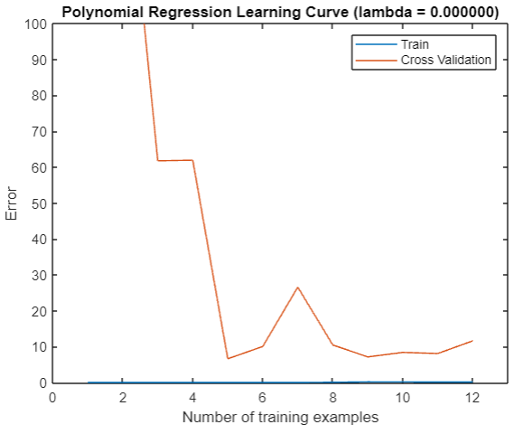
It can be seen that our training error has always been 0, but the verification error is not small.

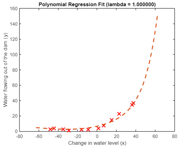
take λ \lambda λ Set to 1, you can clearly see the improvement of fitting:

% Choose the value of lambda
lambda = 1;
[theta] = trainLinearReg(X_poly, y, lambda);

% Plot training data and fit
plot(X, y, 'rx', 'MarkerSize', 10, 'LineWidth', 1.5);
plotFit(min(X), max(X), mu, sigma, theta, p);
xlabel('Change in water level (x)');
ylabel('Water flowing out of the dam (y)');
title (sprintf('Polynomial Regression Fit (lambda = %f)', lambda));

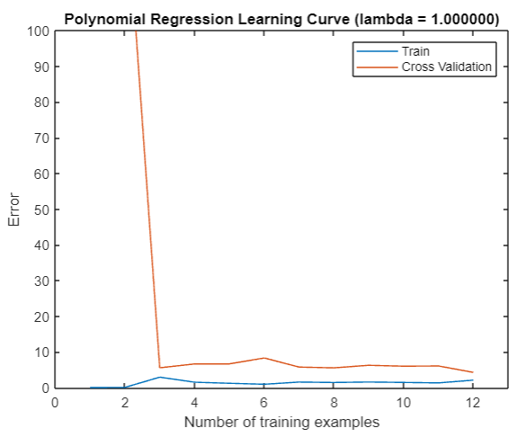
plot(1:m, error_train, 1:m, error_val);
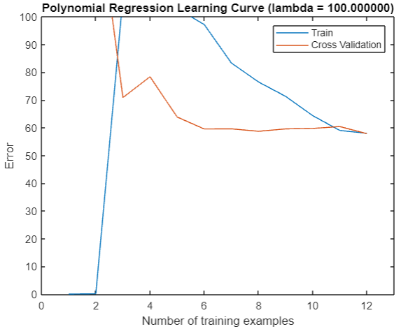
title(sprintf('Polynomial Regression Learning Curve (lambda = %f)', lambda));
xlabel('Number of training examples')
ylabel('Error')
axis([0 13 0 100])
legend('Train', 'Cross Validation')

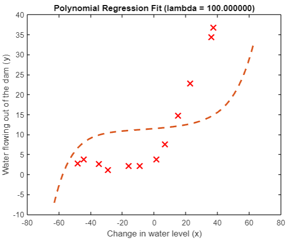
take λ \lambda λ Change it to 100, and the problem appears again. It is obvious that we are out of line:


So how do we choose the regular parameter? Is there a better one than 1 λ \lambda λ？

Select appropriate regular parameters

We can use Divide training set, verification set and test set First list a series of methods λ \lambda λ， Train in the training concentration, put the model in the verification concentration to see who is the best, and take the best to the test concentration to try whether it has been fitted.

function [lambda_vec, error_train, error_val] = ...
    validationCurve(X, y, Xval, yval)
%VALIDATIONCURVE Generate the train and validation errors needed to
%plot a validation curve that we can use to select lambda
%   [lambda_vec, error_train, error_val] = ...
%       VALIDATIONCURVE(X, y, Xval, yval) returns the train
%       and validation errors (in error_train, error_val)
%       for different values of lambda. You are given the training set (X,
%       y) and validation set (Xval, yval).
%

% Selected values of lambda (you should not change this)
lambda_vec = [0 0.001 0.003 0.01 0.03 0.1 0.3 1 3 10]';

% You need to return these variables correctly.
error_train = zeros(length(lambda_vec), 1);
error_val = zeros(length(lambda_vec), 1);

% ====================== YOUR CODE HERE ======================
% Instructions: Fill in this function to return training errors in 
%               error_train and the validation errors in error_val. The 
%               vector lambda_vec contains the different lambda parameters 
%               to use for each calculation of the errors, i.e, 
%               error_train(i), and error_val(i) should give 
%               you the errors obtained after training with 
%               lambda = lambda_vec(i)
%
% Note: You can loop over lambda_vec with the following:
%
%       for i = 1:length(lambda_vec)
%           lambda = lambda_vec(i);
%           % Compute train / val errors when training linear 
%           % regression with regularization parameter lambda
%           % You should store the result in error_train(i)
%           % and error_val(i)
%           ....
%           
%       end
%
%
for i=1:length(lambda_vec)
    lambda=lambda_vec(i);
    [theta]=trainLinearReg(X, y, lambda);
    [error_train(i)]=linearRegCostFunction(X,y,theta,0);
    [error_val(i)]=linearRegCostFunction(Xval,yval,theta,0);
end

% =========================================================================

end

In this way, we can get a price- λ \lambda λ Curve:

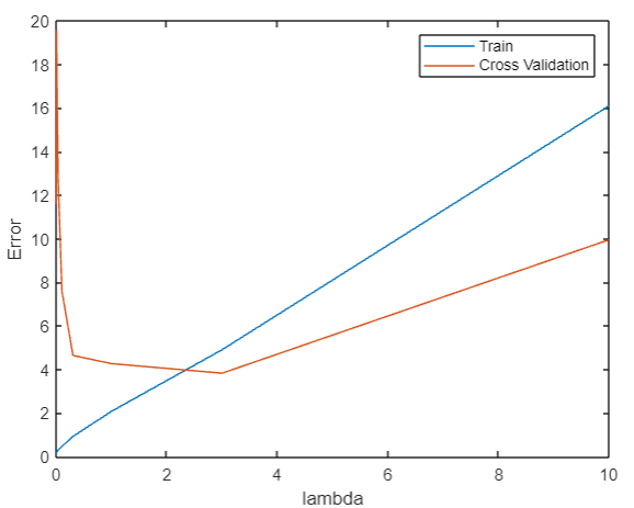
It can be found that in λ = 3 \lambda=3 λ= At 3:00, the cost of verification is the least. Put it into the test set:

lambda=3;
[theta]=trainLinearReg(X_poly, y, lambda);
fprintf("%f\n",linearRegCostFunction(X_poly_test,ytest,theta,0));

The cost is 3.8599, which shows that our fitting is quite appropriate.